Lecture 9: Feature Descriptors

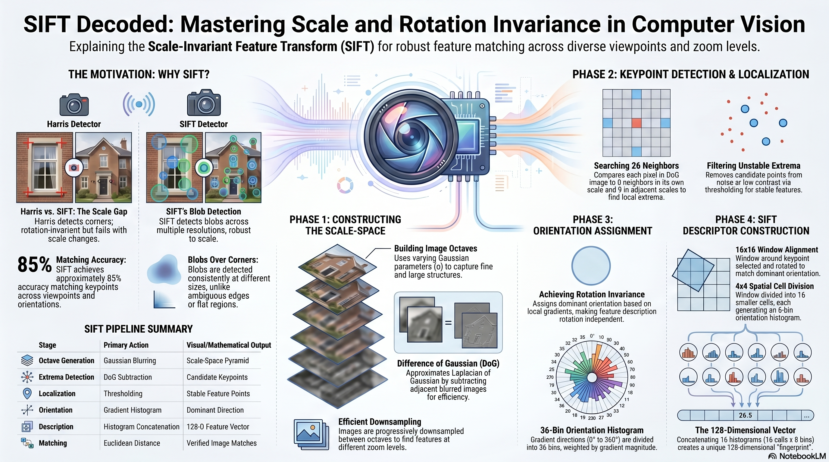
Why Do We Need Feature Detection?

Identifying distinctive locations for matching across images

Feature detection is an essential step in computer vision because it allows us to identify distinctive image locations that can be described mathematically and matched across different images. Feature detection is required when we want to describe image structures such as fingerprints, corners, or blobs in a compact mathematical representation. Feature detection also enables matching the same object across multiple images even if the object appears at different orientations or scales. For example, if we highlight a bell in one image and attempt to locate the same bell in another rotated or resized image, we cannot rely on raw pixel comparison alone. Instead, we must detect distinctive interest points that remain stable under geometric transformations.

Main Challenge in Feature Matching

The main difficulty is allowing the computer to automatically detect corresponding objects across different images without manual intervention. Instead of comparing entire images directly, it is better to detect unique local features and match those between images. These detected features must remain stable even when the object undergoes transformations such as scaling or rotation. A simple distance function between pixel intensities is usually insufficient because it is highly sensitive to geometric transformations. Therefore, robust feature detection methods must be invariant to orientation and scale.

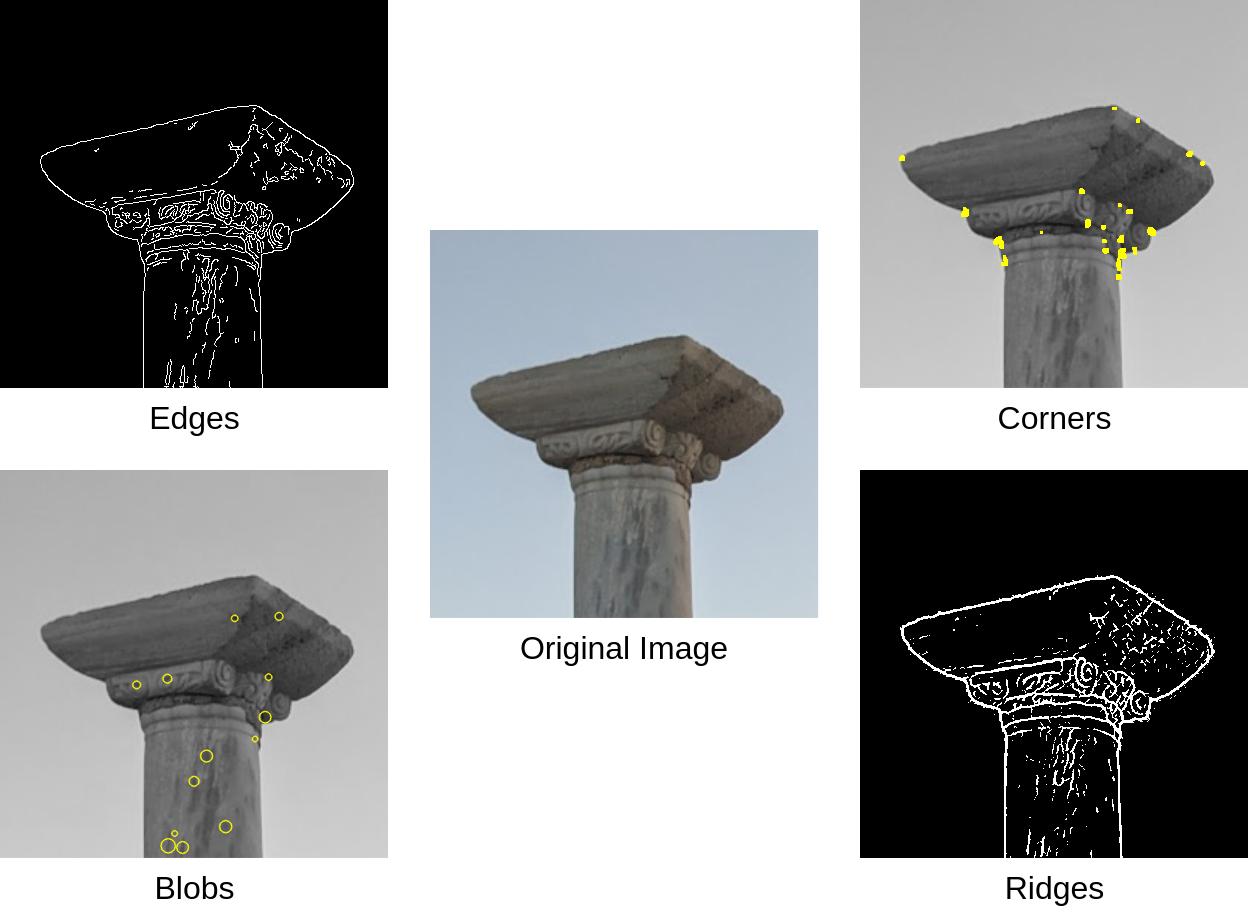
Which Features Are Most Reliable?

Different image structures respond differently to geometric transformations, and not all structures are equally useful for matching.

Flat Regions

Little intensity variation

Cannot be uniquely identified

Not useful

Edges

More informative than flat

Ambiguous along edge direction

Partially useful

Corners

Reliable local structures

Detected by Harris detector

Good — not scale-invariant

Blobs

Groups of similar pixels

Detectable across scales

Best for multi-scale matching

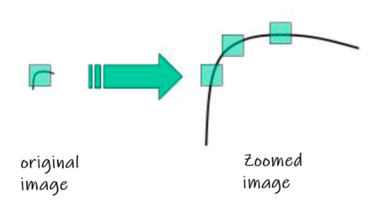
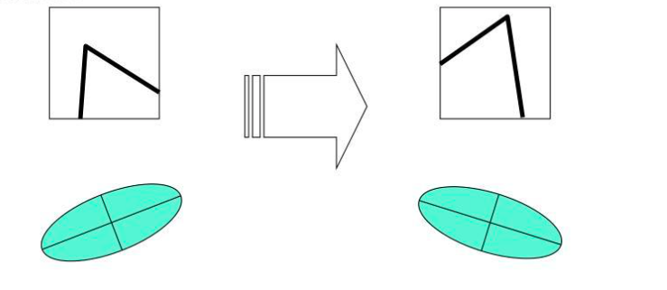
Harris Detector — Rotation Invariant but NOT Scale Invariant

✓ Rotation Invariant

Relies on eigenvalues of structure tensor

Eigenvalues unchanged after rotation

Ellipse rotates; eigenvalues stay the same

Same corner detected at any orientation

✗ NOT Scale Invariant

Window size is fixed — never changes

Same corner at different zoom looks different

Detection inconsistent across resolutions

This limitation motivates SIFT

When an image is zoomed, the same corner appears at a different apparent size, and a detector with a fixed window size may fail to detect it consistently — illustrating that Harris is not scale-invariant. When the image rotates, the ellipse representing the structure tensor rotates accordingly while its eigenvalues remain unchanged — so Harris handles rotation but not scale.

What is SIFT?

Scale-Invariant Feature Transform (SIFT)

SIFT is a feature detection and description algorithm designed to identify image structures across multiple scales and orientations. SIFT detects image features known as blobs instead of relying only on corners. A blob is a group of connected pixels that share similar intensity properties. Instead of detecting blob boundaries, SIFT uses blob responses to guide the selection of stable interest points. These detected points remain consistent even under scaling and rotation transformations.

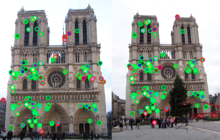
SIFT Matching Performance & Applications

Lecture example: ~85%

Example result: 85 correct, 15 incorrect out of 100

Robust to viewpoint, scale, orientation changes

Applications

Object recognition

Image stitching & panoramas

3D reconstruction

Augmented reality

SIFT Handles

Scale changes (zoom in / out)

Rotation changes

Moderate illumination shifts

Moderate viewpoint changes

Detecting Features Across Multiple Scales

SIFT searches for stable image features by exploring structures at different spatial resolutions. The algorithm examines blobs at several scales instead of using a single fixed window size. This allows the detector to identify features that appear small in one image and large in another. The goal is to locate characteristic regions whose responses remain strong across multiple scales.

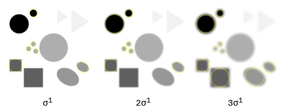
Scale Invariance Using Laplacian of Gaussian (LoG)

Maximum response when filter scale matches blob size

Scale selection is motivated by the scale-normalized Laplacian of Gaussian (LoG). Its response has an extremum at a blob center when the filter scale matches the blob's characteristic size. Varying \(\sigma\) therefore detects structures of different sizes. SIFT computes the cheaper Difference of Gaussians rather than evaluating LoG directly.

\[ \operatorname{LoG}_{\mathrm{norm}}(x,y,\sigma)=\sigma^2\nabla^2G(x,y,\sigma), \qquad \nabla^2=\frac{\partial^2}{\partial x^2}+\frac{\partial^2}{\partial y^2} \] \[ G(x,y,\sigma)=\frac{1}{2\pi\sigma^2} \exp\!\left(-\frac{x^2+y^2}{2\sigma^2}\right) \]

For an ideal circular Gaussian blob of radius r: sigma approximately r / sqrt(2), equivalently r approximately sqrt(2) sigma. Edge localization: zero-crossings of a Laplacian response. Blob localization: extrema of the scale-normalized LoG/DoG response. The extremum may be positive or negative depending on blob polarity.

Small σ (fine scale)

Fine image details preserved

Detects small blobs

High spatial frequency structures

Large σ (coarse scale)

Heavy blurring applied

Detects large blobs

Low spatial frequency structures

Blob Detection Using LoG Responses

Blob detection is similar to edge detection, but the objective is different. Edge detection identifies zero-crossings of the Laplacian response. Blob detection identifies maxima of the Laplacian response. The maximum response occurs when the filter scale matches the blob scale. Therefore, selecting the correct σ allows accurate blob localization.

Difference of Gaussian (DoG) — Efficient Approximation of LoG

DoG ≈ LoG — computationally much cheaper

In practice, SIFT approximates the Laplacian of Gaussian using the Difference of Gaussian operator. The Difference of Gaussian is computed by subtracting two Gaussian-blurred images with different σ values. The parameter σ in the Gaussian filter controls the amount of image blurring. Small values of σ preserve fine image details, while large values of σ emphasize larger structures. This approximation significantly reduces computational complexity. Despite being simpler, DoG preserves strong responses at blob centers. Therefore, DoG is widely used for efficient multi-scale feature detection.

\[ L(x,y,\sigma)=G(x,y,\sigma)*I(x,y) \] \[ D(x,y,\sigma)=L(x,y,k\sigma)-L(x,y,\sigma) =\bigl(G(x,y,k\sigma)-G(x,y,\sigma)\bigr)*I(x,y) \] \[ D(x,y,\sigma)\approx (k-1)\sigma^2\nabla^2G(x,y,\sigma)*I(x,y), \qquad k=2^{1/S} \]

S is the number of scale intervals per octave. Thus k = sqrt(2) only when S = 2; the common canonical choice S = 3 gives k = 2^(1/3).

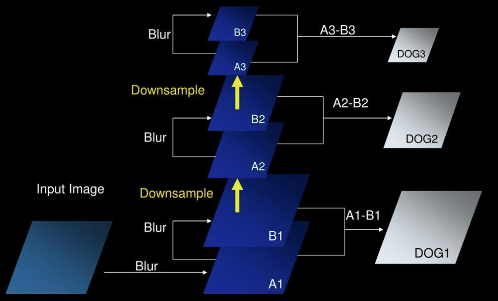
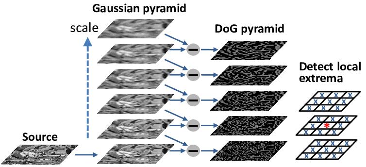
DoG Pyramid — Level by Level

Level 1: Input Image → Blur → A1 → Blur → B1 (A1 − B1 → DoG1) Level 2: B1 → Downsample → A2 → Blur → B2 (A2 − B2 → DoG2) Level 3: B2 → Downsample → A3 → Blur → B3 (A3 − B3 → DoG3) Each DoG level captures blob-like structures at a different spatial resolution.

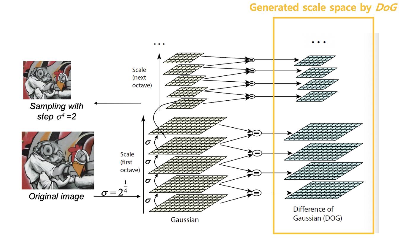
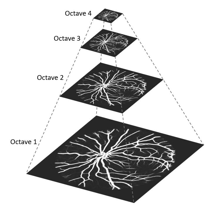
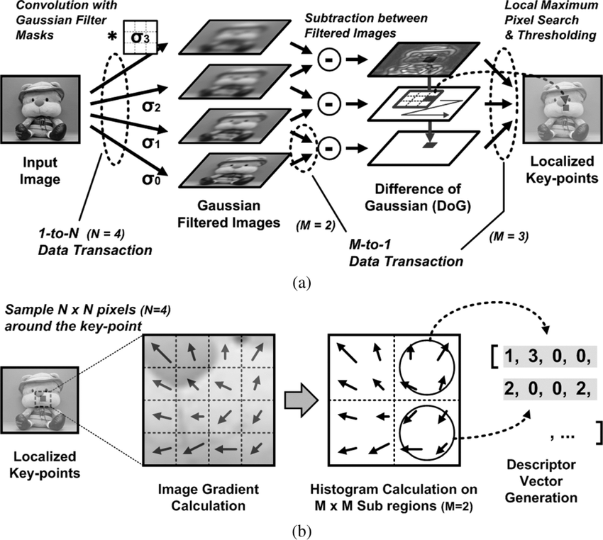
Building Octaves (Step 0 of SIFT)

The first step of SIFT is constructing a Gaussian scale space. An octave covers a doubling of \(\sigma\) at one image resolution; adjacent scales differ by \(k=2^{1/S}\). After one octave, an appropriately blurred Gaussian image is downsampled by two to begin the next octave. The lecture illustrates this idea with four Gaussian levels. In canonical SIFT, \(S\) usable intervals require \(S+3\) Gaussian images and \(S+2\) DoG images per octave so that 3-level extrema comparisons are available at the boundaries. With the common \(S=3\), that is 6 Gaussian and 5 DoG images.

Octave 1

Full-resolution image

Lecture illustration: 4 Gaussian levels

Canonical SIFT (S=3): 6 Gaussian, 5 DoG

Octave 2

Downsampled by 2×

Same scale schedule at half resolution

Each octave spans a 2x change in sigma

Octave 3, 4…

Downsampled again 2×

Same structure per octave

Captures coarser structures

Why Octaves?

By downsampling between octaves, SIFT covers a very wide range of scales efficiently. A blob that is 2× larger in the original image is captured at the same relative scale in the next octave. This is computationally cheaper than simply increasing σ indefinitely.

SIFT Algorithm — 4 Main Processing Steps

Step 1_{Scale-Space Extrema}

→

Step 2_{Keypoint Localization}

→

Step 3_{Orientation Assignment}

→

Step 4_{128-D Descriptor}

Detection of scale-space extrema using the Difference-of-Gaussian pyramid. Candidate keypoints are identified as local maxima or minima across both spatial and scale dimensions.

Keypoint localization and filtering. Weak or unstable extrema caused by noise or low contrast are removed using thresholding. Interpolation refines keypoint position and scale.

Orientation assignment using gradient histograms. A dominant orientation is assigned to each keypoint to achieve rotation invariance.

Construction of a distinctive 128-dimensional descriptor for each keypoint using local gradient orientation histograms.

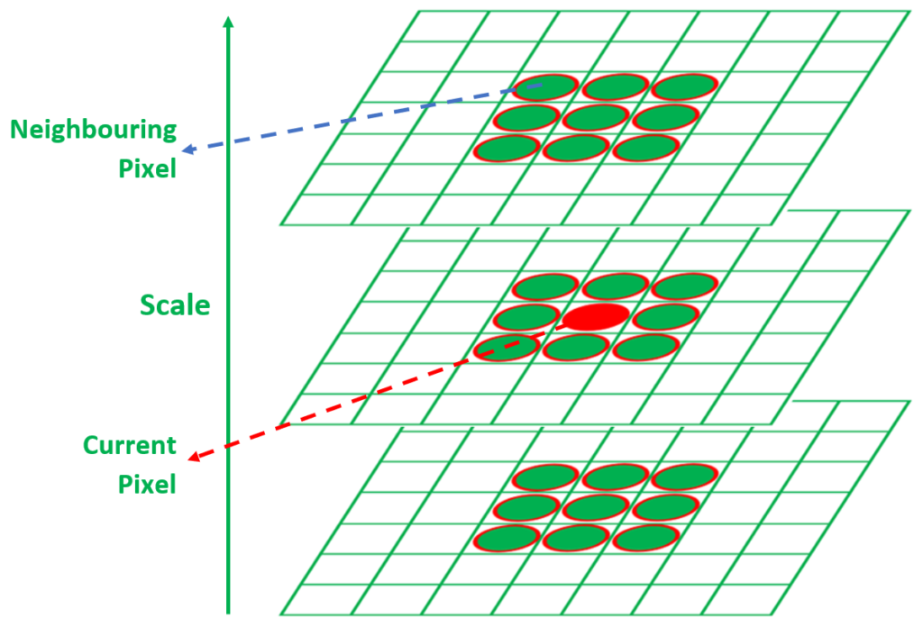
Step 1 — Detecting Scale-Space Extrema

Comparing each pixel to 26 neighbors across 3 scale levels

Candidate keypoints are detected by searching for extrema across spatial and scale dimensions. Each pixel is compared with its neighbors in the same image and adjacent scales. Each pixel in a DoG image is compared with its 8 neighboring pixels in the same scale, 9 neighboring pixels in the scale above, and 9 neighboring pixels in the scale below.

For each pixel in a DoG image, compare with: Same scale level : 8 neighboring pixels (3×3 window minus center) Scale above : 9 neighboring pixels (full 3×3 grid) Scale below : 9 neighboring pixels (full 3×3 grid) ──────────────────────────────────────── Total comparisons: 8 + 9 + 9 = 26 surrounding values A pixel is selected as a candidate keypoint if: it is GREATER than all 26 neighbors (local maximum), OR it is LESS than all 26 neighbors (local minimum) These extrema correspond to candidate blob centers that remain stable across spatial and scale dimensions.

A sample \(D(x,y,\sigma)\) is a candidate only if it is strictly larger than all 26 neighbors or strictly smaller than all 26 neighbors: 8 at \(\sigma\), 9 at \(k\sigma\), and 9 at \(\sigma/k\).

Why compare across scales?

By searching for extrema in both spatial dimensions AND scale, SIFT finds points that are distinctive not just locally in the image, but also at a specific characteristic scale. This gives each keypoint a natural scale that can be used to make the descriptor scale-invariant.

Step 2 — Keypoint Localization

After detecting candidate extrema, weak or unstable keypoints must be removed. Some detected extrema occur due to noise or low contrast — these points are eliminated using thresholding. Interpolation is applied to estimate more accurate values of σ. Only stable extrema are retained as final feature points.

Removed by thresholding

Low contrast extrema (noise-induced)

Extrema on edge structures (poorly localized)

Unstable responses that shift with perturbations

Retained as final keypoints

High contrast, stable extrema only

Strong DoG response at blob centers

Position refined using interpolation

Subpixel and Subscale Refinement

SIFT fits a three-dimensional quadratic to the local DoG samples. This refines the keypoint's image coordinates and scale beyond the discrete pyramid samples. Here \(\mathbf{x}=(\Delta x,\Delta y,\Delta\sigma)^T\) is the offset from the sampled candidate.

\[ D(\mathbf{x})\approx D+ \left(\frac{\partial D}{\partial\mathbf{x}}\right)^T\mathbf{x} +\frac{1}{2}\mathbf{x}^T \frac{\partial^2D}{\partial\mathbf{x}^2}\mathbf{x} \] \[ \mathbf{x}^{*}=-\left(\frac{\partial^2D}{\partial\mathbf{x}^2}\right)^{-1} \frac{\partial D}{\partial\mathbf{x}}, \qquad D(\mathbf{x}^{*})=D+\frac{1}{2} \left(\frac{\partial D}{\partial\mathbf{x}}\right)^T\mathbf{x}^{*} \]

Reject a low-contrast candidate when |D(x*)| is below the selected contrast threshold (0.03 in the reference formulation used by this guide).

Rejecting Edge-Like Responses

A strong DoG response along an edge can be poorly localized across the edge. SIFT examines the 2D spatial Hessian at the refined scale. If one principal curvature is much larger than the other, the candidate is edge-like and is rejected.

\[ H=\begin{bmatrix}D_{xx}&D_{xy}\\D_{xy}&D_{yy}\end{bmatrix},\qquad \operatorname{Tr}(H)=D_{xx}+D_{yy}=\alpha+\beta, \qquad \det(H)=D_{xx}D_{yy}-D_{xy}^{2}=\alpha\beta \] \[ \frac{\operatorname{Tr}(H)^2}{\det(H)} <\frac{(r_{\mathrm{th}}+1)^2}{r_{\mathrm{th}}} \]

The canonical curvature-ratio threshold is r_th = 10. Reject when det(H) is non-positive or when the ratio is at least the bound; retain only well-localized extrema.

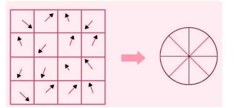
Step 3 — Orientation Assignment

Achieving rotation invariance via gradient histograms

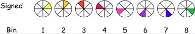
Each detected keypoint is assigned a dominant orientation so that the descriptor remains stable when the image rotates. A neighborhood around the detected keypoint is selected from the corresponding octave and scale level. For each pixel in this neighborhood, the gradient magnitude and gradient direction are computed using intensity differences in the horizontal and vertical directions. Each pixel contributes a vote to an orientation histogram according to its gradient direction. The votes are weighted by gradient magnitude so that stronger edges contribute more strongly than weaker ones. The orientation range from 0° to 360° is divided into 36 bins to achieve accurate estimation of the dominant orientation of the keypoint. The bin with the largest accumulated votes defines the dominant orientation.

\[ m(x,y)=\sqrt{\bigl(L(x+1,y)-L(x-1,y)\bigr)^2+ \bigl(L(x,y+1)-L(x,y-1)\bigr)^2} \] \[ \theta(x,y)=\operatorname{atan2}\!\left( L(x,y+1)-L(x,y-1),\;L(x+1,y)-L(x-1,y)\right) \]

Use atan2 rather than a one-argument arctangent so the full 0-to-360-degree quadrant is retained. Votes are weighted by magnitude and by a Gaussian window.

Select a neighborhood around the keypoint at the correct octave and scale level.

For each pixel, compute gradient magnitude and direction using horizontal and vertical intensity differences.

iii

Each pixel votes for an orientation bin according to its gradient direction. Votes are weighted by gradient magnitude and a Gaussian centered on the keypoint, reducing the influence of distant samples.

The 0°–360° range is divided into 36 bins (10° each). The bin with the largest accumulated vote is the dominant orientation.

Every local peak at least 80% of the dominant peak creates another keypoint at the same location and scale with that orientation. This is a peak test, not a test of every individual bin.

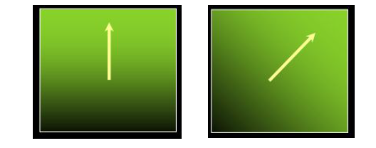
Understanding Gradient Directions Around the Keypoint

Each arrow represents the gradient direction at one pixel inside the keypoint neighborhood. The arrow direction indicates where the image intensity increases most rapidly at that pixel location. The arrow length represents the gradient magnitude, which determines the strength of its vote in the histogram. Accumulating these votes produces the histogram used to estimate the dominant orientation.

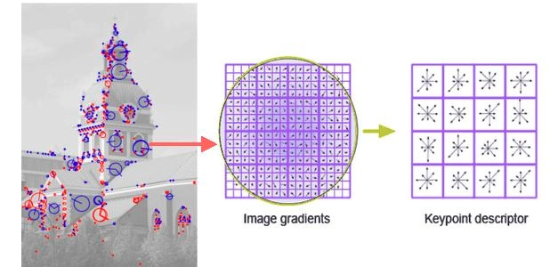
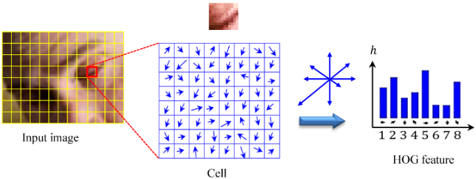
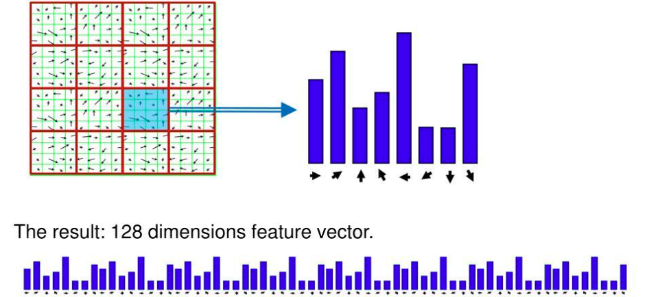
Step 4 — Building the 128-Dimensional SIFT Descriptor

16×16 window → 4×4 cells × 8 orientation bins = 128 values

After assigning the dominant orientation, the local image region is described using multiple smaller orientation histograms. A 16×16 window is selected around the keypoint at the correct scale determined from the DoG pyramid. This window is aligned according to the dominant orientation to achieve rotation invariance. The window is divided into 4×4 smaller spatial cells. For each cell, an orientation histogram with 8 bins is computed covering directions from 0° to 360°. Each pixel contributes to a histogram bin according to its gradient direction, and the contribution is weighted by the gradient magnitude.

\[ 4\times4\ \text{cells}\times8\ \text{orientation bins} =16\times8=128\ \text{dimensions} \]

Standard teaching layout: a 16 x 16 sample window, rotated relative to the keypoint's dominant orientation, divided into 4 x 4 cells (4 x 4 samples per cell). Each sample's vote is distributed by its relative orientation and weighted by gradient magnitude and a Gaussian window. Practical SIFT also interpolates votes between nearby spatial cells and orientation bins to reduce boundary sensitivity.

Descriptor Normalization for Illumination Robustness

For the concatenated vector \(\mathbf{v}\in\mathbb{R}^{128}\): \[ \mathbf{v}_1=\frac{\mathbf{v}}{\lVert\mathbf{v}\rVert_2},\qquad \mathbf{v}_2[i]=\min\!\bigl(\mathbf{v}_1[i],0.2\bigr),\qquad \widehat{\mathbf{v}}=\frac{\mathbf{v}_2}{\lVert\mathbf{v}_2\rVert_2} \]

Unit normalization reduces sensitivity to overall contrast. Clipping at 0.2 limits large gradient peaks caused by nonlinear illumination, then re-normalization restores unit length.

Lecture's Simplified Descriptor Example

Do not confuse the classroom illustration with standard 128-D SIFT

The final pipeline diagram in the original lecture samples a \(4\times4\) neighborhood and divides it into \(2\times2\) subregions. With 8 orientation bins per subregion, that pedagogical descriptor has \(2\times2\times8=32\) values. It demonstrates the same construction principle at a smaller size; the standard descriptor described above has 128 values.

Understanding Each Cell's Histogram

Each arrow inside a cell represents the gradient direction of one pixel. Pixels with similar gradient directions contribute to the same orientation bin. Stronger gradients contribute larger values to the histogram than weaker gradients. These local histograms describe the spatial distribution of intensity changes around the keypoint. The 8 orientation bins cover directions 0°, 45°, 90°, 135°, 180°, 225°, 270°, 315°.

Interactive 4×4 Cell Grid — Click Any Cell

16×16 window → 4×4 cells. Click any cell:

Each cell = 4×4 pixels, 8-bin histogram

Click a cell to see its orientation histogram

0°45°90°135°180°225°270°315°

Why the SIFT Descriptor is Robust

Illumination robustness: Gradients remove additive brightness shifts; normalization reduces multiplicative contrast changes; clipping large entries limits nonlinear effects. This is robustness, not perfect invariance to arbitrary lighting.

Spatial structure preservation: Dividing the region into smaller spatial cells preserves the geometric structure of the neighborhood around the keypoint.

Rotation invariance: Aligning the descriptor with the dominant orientation ensures the descriptor is the same regardless of how the image is rotated.

Scale invariance: Detecting keypoints across multiple octaves and computing the descriptor at the keypoint's characteristic scale ensures scale-invariant description.

Constructing the SIFT Descriptor Vector

Each pixel votes for one orientation bin according to its gradient direction. The vote added to the bin equals the pixel's gradient magnitude (stronger edges contribute more). After all pixels in the cell vote, the bin values form the orientation histogram representing that cell. These histograms capture both the direction and the spatial distribution of intensity changes around the keypoint. Concatenating all histograms produces a compact numerical representation that uniquely characterizes the local image structure.

128-D descriptor breakdown

4 rows × 4 columns = 16 spatial cells. Each cell has an 8-bin orientation histogram. Concatenating all 16 histograms: 16 × 8 = 128 values. This single 128-dimensional vector uniquely characterizes the local image structure around the keypoint and can be reliably matched between different images.

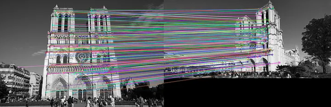
From Blob Detection to Feature Matching in SIFT

The histograms from all subregions are combined to form a 128-dimensional descriptor vector representing the keypoint. Keypoints from different images are matched by comparing their descriptor vectors using a distance measure such as Euclidean distance. Ambiguous matches are removed using the Lowe ratio test, which compares the closest and second-closest descriptor matches. Similar descriptors indicate that the corresponding blobs represent the same physical structure in both images.

\[ d(\mathbf{d}_A,\mathbf{d}_B)= \sqrt{\sum_{i=1}^{128}\left(d_A[i]-d_B[i]\right)^2} \]

Lower distance means more similar descriptors. Nearest-neighbor distance alone can still be ambiguous, so SIFT compares the best candidate with the second-best candidate.

Lowe Ratio Test — Removing Ambiguous Matches

Comparing the closest match to the second-closest match

The ratio test compares the distance to the closest matching descriptor (d1) against the distance to the second-closest matching descriptor (d2). If d1 / d2 is small, the best match is clearly better than the next best — a reliable match. If d1 / d2 is large (close to 1), the two candidates are nearly equally similar — an ambiguous match that should be discarded.

\[ \operatorname{ratio}=\frac{d_1}{d_2},\qquad \text{accept if }\frac{d_1}{d_2}<\tau \]

d1 = distance to the closest neighbor; d2 = distance to the second-closest neighbor. A ratio near 0 means the best match is distinctive; a ratio near 1 means ambiguity. The original SIFT paper used 0.8 in its reported experiments; applications may tune tau.

Interactive Lowe Ratio Simulator

d1 (best match distance)60

d2 (2nd best distance)120

Threshold0.75

d1 (best match)

d2 (2nd best match)

Full SIFT Pipeline Summary

Gaussian Pyramid_{Build octaves}

→

DoG Extrema_{Find candidates}

→

Keypoint Localization_{Remove unstable}

→

Orientation_{36-bin histogram}

→

128-D Descriptor_{4x4 cells x 8 bins}

→

Match + Lowe_{Euclidean + ratio}

Comparison — Harris vs SIFT

Property	Harris	SIFT
Feature type	Corners	Blobs
Scale invariant	No (fixed window)	Yes (multi-scale DoG)
Rotation invariant	Yes (eigenvalues)	Yes (orientation alignment)
Descriptor	None (detection only)	128-D gradient histogram
Scale selection	Manual	Automatic via DoG extrema
Orientation assigned	No	Yes — dominant gradient direction
Matching method	N/A	Euclidean distance + Lowe test
Applications	Basic corner detection	Matching, stitching, 3D reconstruction

Scale-Space Explorer

Adjust canonical scale-space parameters. For \(S\) intervals per octave, SIFT stores \(S+3\) Gaussian images and \(S+2\) DoG images so interior DoG levels can be compared above and below.

Number of octaves3

Intervals per octave (S)3

Base σ (σ₀)1.0

Descriptor Dimension Calculator

Window size (N×N)16

Cell grid (M×M)4

Orientation bins8

26-Neighbor Extrema Detection — Breakdown

Scale-space extrema search neighborhood: Same scale level : 3×3 window − 1 center = 8 neighbors Scale above : 3×3 window = 9 neighbors Scale below : 3×3 window = 9 neighbors ───────────────────────────────── Total : 8 + 9 + 9 = 26 neighbors A pixel is a candidate keypoint ONLY if it is: • GREATER than all 26 neighbors (local maximum), OR • LESS than all 26 neighbors (local minimum) This strict requirement ensures only truly distinctive blob-center candidates are selected as keypoints.

Orientation Histogram Bins

Orientation assignment histogram: Range : 0° to 360° Bins : 36 (one every 10°) Weight : each pixel's vote = its gradient magnitude Dominant orientation = bin with highest accumulated weight Multiple orientation rule: If another bin has ≥ 80% of the maximum bin's value, a second (or third) orientation is also assigned. This creates multiple keypoints at the same spatial location but with different orientations — improving matching robustness.