Visual Cheat Sheet Summary
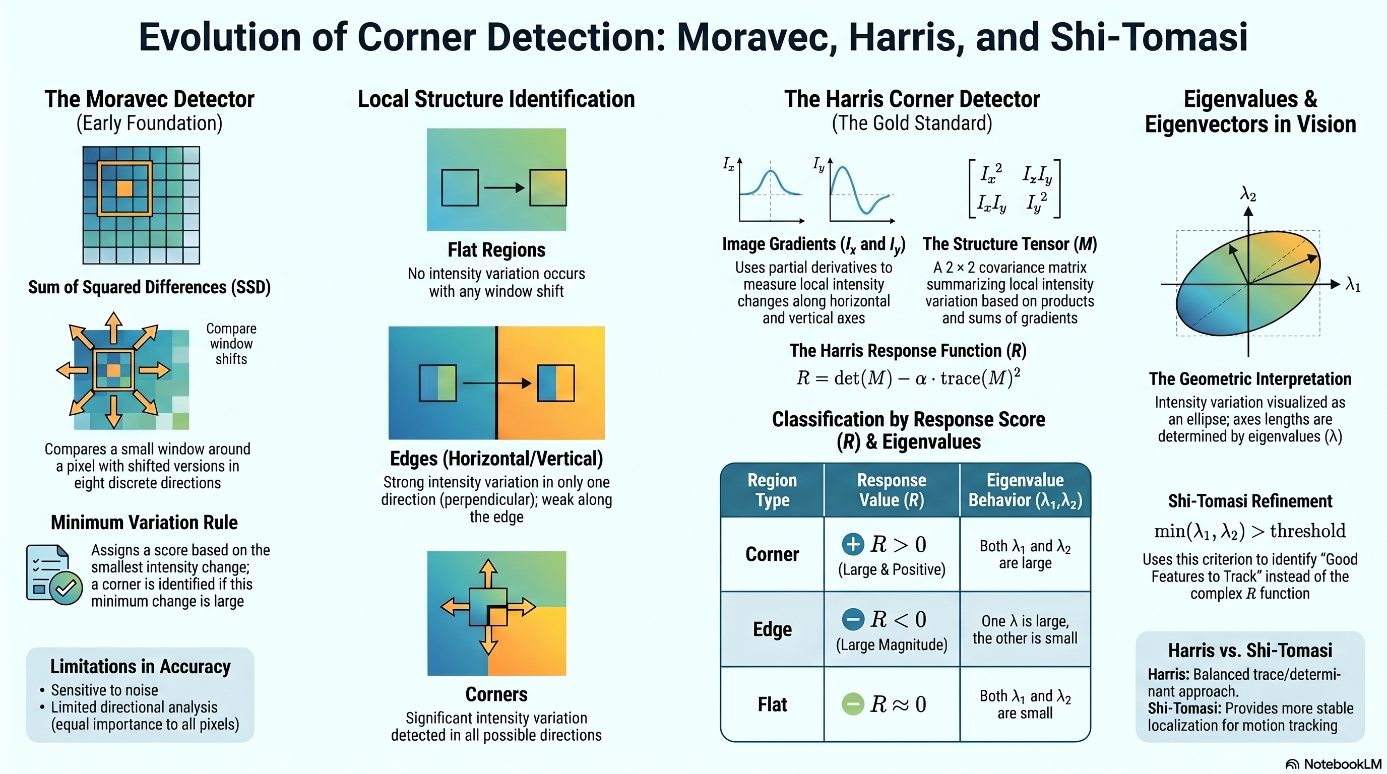
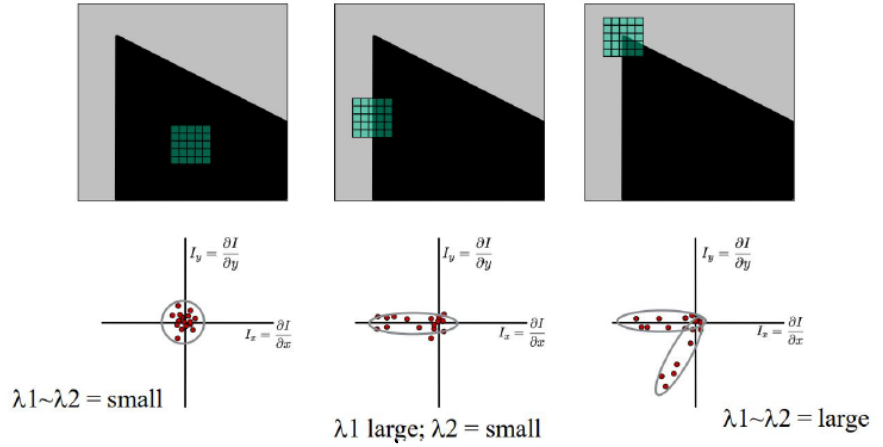
1-Image Summary
50-Question Practice Quiz
This comprehensive practice quiz contains 50 multiple-choice questions loaded directly from the lecture database.
What is the Moravec Corner Detector?
Earliest corner detection algorithm — measuring intensity variation
For each pixel at position (m, n), a small window is centered around it and compared with shifted versions of the same window in different directions. The intensity variation between the original window and each shifted window is measured using the Sum of Squared Differences (SSD). The minimum SSD among all directions is assigned as the score $F_{m,n}$ for that pixel. Corner points are pixels where this minimum SSD is locally large compared to neighbors.
Mathematical Formulation
Sum of Squared Differences (SSD) for shift \((x,y)\): \[E_{m,n}(x,y) = \sum_{u,v} w_{m,n}(u,v) \left[ f(u+x, v+y) - f(u,v) \right]^2\] where: • \(f(u,v)\) = intensity at pixel \((u, v)\) • \((x, y)\) = shift direction applied to window • \(w_{m,n}(u,v)\) = weighting window centered at pixel \((m, n)\) (uniform rectangular for Moravec) Moravec Corner Response Score: \[F_{m,n} = \min_{(x,y) \in \mathcal{D}} E_{m,n}(x,y)\] Direction Set \(\mathcal{D}\): \[\mathcal{D} = \{ (1,0), (-1,0), (0,1), (0,-1), (1,1), (-1,-1), (1,-1), (-1,1) \}\] Corresponding to shifts of one pixel in the eight principal directions (horizontal, vertical, and diagonal).
Detection Steps
1
Center a small square window around the pixel under examination.
2
Shift the window by one pixel in several directions: up, down, left, right, and all four diagonal directions.
3
For each shift direction, compute the Sum of Squared Differences (SSD) between the original and shifted windows.
4
Select the smallest SSD value among all eight shift directions as the variation measure for that pixel.
5
Pixels whose variation values exceed a predefined threshold and are local maxima are classified as corner points.
Local Structures — Interpretation

Flat Region

SSD behavior: Small in all directions
Minimum SSD: Low → pixel is not a corner
Intensity barely changes when window shifts in any direction

Vertical Edge

SSD behavior: Large horizontal, small vertical
Minimum SSD: Low (dominated by small direction)
Window can slide along edge without much change

Horizontal Edge

SSD behavior: Large vertical, small horizontal
Minimum SSD: Low (dominated by small direction)
Same issue — minimum is small despite some large SSD

Corner

SSD behavior: Large in ALL directions
Minimum SSD: High → pixel IS a corner
Intensity changes significantly no matter which direction you shift
Corner Selection Using Thresholding
After computing the minimum SSD for every pixel in the image, a threshold is applied. Pixels whose SSD values exceed the threshold are classified as corners. For example, if the threshold is chosen as 2, all pixels with minimum SSD \(\ge 2\) are detected as corners.
Worked Example — Corner Detection at Pixel (3,3)
SSD Calculations for Binary Object/Background Intersection
Consider a simplified image containing only two intensity values: black pixels (0) and gray pixels (128). Let's trace how the detector evaluates candidate pixel \((3,3)\) centered inside a local window:

Selecting the Reference Sub-Image: A small square window is centered around pixel \((3,3)\).
Evaluating Shifts: The window is shifted by one pixel in multiple directions (such as upward, leftward, and diagonally).
Computing SSDs: For each shift, the Sum of Squared Differences is calculated by computing the squared differences between corresponding pixel intensities in the original and shifted windows:
1. Shift Upward: \(\text{SSD}_{\text{up}} = \sum \left[ f(u, v - 1) - f(u,v) \right]^2\) 2. Shift Leftward: \(\text{SSD}_{\text{left}} = \sum \left[ f(u - 1, v) - f(u,v) \right]^2\) 3. Shift Diagonally: \(\text{SSD}_{\text{diag}} = \sum \left[ f(u - 1, v - 1) - f(u,v) \right]^2\)
Result: Since the window overlaps a corner, shifting in any of the directions results in significant intensity differences. Consequently, the SSD values in all directions (horizontal, vertical, and diagonal) are large, yielding a high minimum SSD score \(F_{3,3}\) which correctly classifies pixel \((3,3)\) as a corner.
Limitations of the Moravec Detector
Why Moravec was eventually replaced
Discrete directionsConsiders only a small number of fixed shift directions (8) instead of analyzing variation continuously in all directions.
Uniform windowAll pixels inside the window are assigned equal importance, reducing detection accuracy in complex regions.
Noise sensitiveSmall intensity fluctuations can produce incorrect corner responses.
Edge confusionRelies only on the minimum SSD, so it can misclassify strong edges as corners when the minimum direction happens to be perpendicular to the edge.
Takeaway
These four limitations motivated the development of the Harris corner detector, which analyzes intensity variation continuously across all directions using gradients and the structure tensor.
Introduction to Harris Corner Detector
Overcoming Moravec's limitations with gradient-based analysis
The Harris detector analyzes intensity changes continuously across all directions rather than evaluating a handful of discrete shifts. It relies on correlations between neighboring pixels inside a local window, captured through image gradients and a covariance (structure tensor) matrix. These allow the detector to robustly distinguish flat regions, edges, and corners.
Core Idea — Continuous Directional Analysis

Moravec approach

8 discrete shift directions
Uniform rectangular window
Takes minimum of SSD values
Noisy, anisotropic response

Harris approach

All continuous directions
Gaussian-weighted window
Structure tensor + eigenvalues
Rotation-invariant, more stable
Role of Covariance in Harris Detector
The Harris detector uses covariance to measure how pixel intensities vary together inside a local region. It captures intensity variation along horizontal and vertical directions simultaneously and how strongly they correlate.

Flat Region

Small variation both directions
Both eigenvalues ≈ 0

Edge

Large in one direction only
One eigenvalue large, one ≈ 0

Corner

Large in BOTH directions
Both eigenvalues large
Derivation — Intensity Variation Function
The change in intensity caused by shifting a window by \((u, v)\) is formulated as: \[E(u,v) = \sum_{x,y} w(x,y) \left[ I(x+u, y+v) - I(x,y) \right]^2\] where: • \(w(x,y)\): Gaussian weighting window centered around the pixel (center pixels weighted more). • \((u,v)\): Small shift offset in any direction.
Taylor Expansion Approximation
To analyze intensity variation continuously, we use a first-order Taylor series expansion to approximate the shifted intensity term: \[I(x+u, y+v) \approx I(x,y) + u I_x + v I_y\] where \(I_x = \frac{\partial I}{\partial x}\) and \(I_y = \frac{\partial I}{\partial y}\) are the partial derivatives of intensity.

Substituting this approximation back into the difference term gives: \[\left[ I(x+u,y+v) - I(x,y) \right]^2 \approx (u I_x + v I_y)^2 = u^2 I_x^2 + 2uv I_x I_y + v^2 I_y^2\] This can be written in matrix quadratic form: \[E(u,v) \approx \begin{bmatrix} u & v \end{bmatrix} M \begin{bmatrix} u \\ v \end{bmatrix}\] where \(M\) is the covariance matrix or structure tensor summarizing the local intensity structure.
Using Partial Derivatives

Horizontal Gradient \(I_x\)

Filter: \(\begin{bmatrix} -1 & 0 & 1 \end{bmatrix}\) applied to each row
\(I_x = \frac{\partial I}{\partial x}\)
\(I_x = \text{right pixel} - \text{left pixel}\)
Example: \(\begin{bmatrix} -1 & 0 & 1 \end{bmatrix} \cdot \begin{bmatrix} 1 & 0 & 5 \end{bmatrix} = -1(1) + 0(0) + 1(5) = 4\)

Vertical Gradient \(I_y\)

Filter: \(\begin{bmatrix} -1 \\ 0 \\ 1 \end{bmatrix}\) applied to each column
\(I_y = \frac{\partial I}{\partial y}\)
\(I_y = \text{bottom pixel} - \text{top pixel}\)
Example: \(\begin{bmatrix} -1 \\ 0 \\ 1 \end{bmatrix}^T \cdot \begin{bmatrix} 1 \\ 5 \\ 9 \end{bmatrix} = -1(1) + 0(5) + 1(9) = 8\)
Structure Tensor Matrix \(M\)
The structure tensor summarizes intensity variation inside the local neighborhood: \[M = \sum_{x,y} w(x,y) \begin{bmatrix} I_x^2 & I_x I_y \\ I_x I_y & I_y^2 \end{bmatrix}\] Where: • Diagonal elements \(I_x^2\) and \(I_y^2\) represent intensity variation along the horizontal and vertical directions respectively. • Off-diagonal elements \(I_x I_y\) represent the correlation between intensity changes along both directions. • \(w(x,y)\) is a Gaussian window that weights central pixels more strongly, making the detector more robust and less sensitive to noise than the uniform rectangular window used in Moravec.
Geometric Interpretation of the Quadratic Form
The quadratic form $E(u,v) \approx [u\ v]\ M\ [u\ v]^T$ describes elliptical contours in the direction space. The shape of those ellipses is determined by the eigenvalues of M:

Circular contours

$\lambda_1 \approx \lambda_2$
Equal variation all directions
→ Corner

Elongated ellipse

$\lambda_1 \gg \lambda_2$
Dominant in one direction
→ Edge

Very flat ellipse

$\lambda_1 \approx \lambda_2 \approx 0$
Almost no variation
→ Flat region
Worked Numerical Example — Pixel (2,2)
5×5 image, 3×3 analysis window around pixel (2,2)
Consider a $5 \times 5$ grayscale image segment. We will analyze the pixel at position \((2,2)\) using a local window of size $3 \times 3$ (highlighted in the center): \[I = \begin{bmatrix} 0 & 0 & 1 & 4 & 9 \\ 1 & 0 & \mathbf{5} & \mathbf{7} & \mathbf{11} \\ 1 & 4 & \mathbf{9} & \mathbf{12} & \mathbf{16} \\ 3 & 8 & \mathbf{11} & \mathbf{14} & \mathbf{16} \\ 8 & 10 & 15 & 16 & 20 \end{bmatrix}\] The centered $3 \times 3$ submatrix corresponds to: \[W = \begin{bmatrix} 5 & 7 & 11 \\ 9 & 12 & 16 \\ 11 & 14 & 16 \end{bmatrix}\]
1
Compute horizontal and vertical gradients using derivative filters \(\begin{bmatrix} -1 & 0 & 1 \end{bmatrix}\) and \(\begin{bmatrix} -1 \\ 0 \\ 1 \end{bmatrix}\) centered at each pixel in the window: \[I_x = \begin{bmatrix} 4 & 7 & 6 \\ 8 & 8 & 7 \\ 8 & 6 & 5 \end{bmatrix}, \quad I_y = \begin{bmatrix} 4 & 8 & 8 \\ 8 & 6 & 7 \\ 6 & 6 & 4 \end{bmatrix}\]
2
Compute gradient products and sums across the window to build the structure tensor \(M\): \[\sum I_x^2 = 4^2 + 7^2 + 6^2 + 8^2 + 8^2 + 7^2 + 8^2 + 6^2 + 5^2 = 403\] \[\sum I_y^2 = 4^2 + 8^2 + 8^2 + 8^2 + 6^2 + 7^2 + 6^2 + 6^2 + 4^2 = 381\] \[\sum I_x I_y = (4)(4) + (7)(8) + (6)(8) + (8)(8) + (8)(6) + (7)(7) + (8)(6) + (6)(6) + (5)(4) = 385\] \[M = \begin{bmatrix} \sum I_x^2 & \sum I_x I_y \\ \sum I_x I_y & \sum I_y^2 \end{bmatrix} = \begin{bmatrix} 403 & 385 \\ 385 & 381 \end{bmatrix}\]
3
Compute Harris response with sensitivity parameter \(\alpha = 0.04\): \[\det(M) = 403 \times 381 - 385^2 = 153543 - 148225 = 5318\] \[\text{trace}(M) = 403 + 381 = 784\] \[R = \det(M) - \alpha \cdot \text{trace}(M)^2\] \[R = 5318 - 0.04 \times (784)^2 = 5318 - 24586.24 = -19268.24\]
4
Classify: Because \(R = -19268.24\) is a large negative value, the gradient variation is strong in only one principal direction. Therefore, this pixel is classified as an EDGE.
Eigenvalues in Image Analysis
Eigenvalues of the structure tensor matrix M describe how strongly image intensity varies along the two principal directions of the local window. They are the key to distinguishing flat regions, edges, and corners without computing full eigendecomposition.
Eigenvalue Intuition
λ₁ ≈ 0, λ₂ ≈ 0 → Flat
Flat
λ₁ ≫ 0, λ₂ ≈ 0 → Edge
Edge
λ₁ ≫ 0, λ₂ ≫ 0 → Corner
Corner
Harris Response Function \(R\)
Instead of computing eigenvalues explicitly, the Harris detector uses a response function based on the determinant and trace of \(M\) — both computable directly from matrix elements: \[R = \det(M) - \alpha \cdot \text{trace}(M)^2\] where: • \(\det(M) = \lambda_1 \lambda_2 = \left(\sum I_x^2\right)\left(\sum I_y^2\right) - \left(\sum I_x I_y\right)^2\) \(\quad \leftarrow\) product of eigenvalues (measures joint variation) • \(\text{trace}(M) = \lambda_1 + \lambda_2 = \sum I_x^2 + \sum I_y^2\) \(\quad \leftarrow\) sum of eigenvalues (measures total variation) • \(\alpha \in [0.04, 0.06]\) (typically 0.04) is a scaling sensitivity parameter.

Why this works:
Corner: Both \(\lambda_1\) and \(\lambda_2\) are large \(\implies \det(M)\) is extremely large, dominating the subtraction term \(\implies R\) is large and positive.
Edge: One eigenvalue is large while the other is small \(\implies \det(M) \approx 0\) while \(\text{trace}(M)\) is large \(\implies -\alpha \cdot \text{trace}(M)^2\) dominates \(\implies R\) is large and negative.
Flat: Both \(\lambda_1\) and \(\lambda_2\) are small \(\implies \det(M) \approx 0\) and \(\text{trace}(M) \approx 0 \implies R \approx 0\).
Classification by R Value

R ≈ 0 → Flat

λ₁ ≈ 0, λ₂ ≈ 0
det ≈ 0, trace ≈ 0
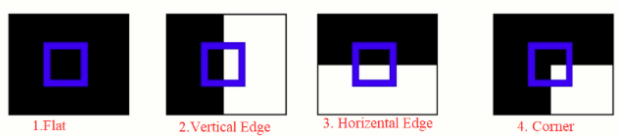
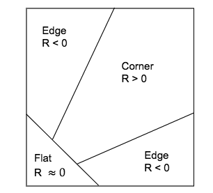
No intensity change in any direction. Not an interest point.

R < 0 → Edge

λ₁ large, λ₂ ≈ 0 (or vice versa)
det ≈ 0, trace large
−α·trace² dominates → R negative. Change in one direction only.

R ≫ 0 → Corner

λ₁ large AND λ₂ large
det large, trace large
det term dominates → R positive. Change in ALL directions.

The Parameter α and Its Role
The constant α balances edge suppression vs. corner detection.

α too small

Edge suppression is weak
Edge points may be falsely detected as corners
Over-detection problem

α too large

Edge suppression is too aggressive
True corners may be missed
Under-detection problem
Recommended value
α = 0.04 is the standard choice, providing a good balance between false edge detections and missed corners. It is determined experimentally and depends on image content and noise level.
Why Eigenvalues Need Not Be Computed Explicitly
One major advantage of the Harris detector: the response function R depends only on det(M) and trace(M), both of which are computable directly from the matrix elements $\Sigma I_x^2$, $\Sigma I_y^2$, $\Sigma I_x I_y$. This avoids the expensive eigenvalue computation and makes the algorithm computationally efficient for real-time applications.
Algorithm Steps — Full Harris Pipeline
1
Compute horizontal and vertical image gradients $I_x$ and $I_y$ using partial derivative filters.
2
For each pixel, construct the structure tensor M from gradient values inside a Gaussian-weighted local window.
3
Compute the Harris response R = det(M) − α·trace(M)² for every pixel.
4
Apply thresholding: pixels with R above threshold → corners, R negative → edges, R ≈ 0 → flat regions.
Computing Eigenvalues When Required
Methods like Shi-Tomasi require explicit eigenvalues of the structure tensor \(M\). These are found by solving the characteristic equation: \[\det(M - \lambda I) = 0\] For a general symmetric $2 \times 2$ covariance matrix \(M = \begin{bmatrix} a & b \\ b & c \end{bmatrix}\): \[\det\left(\begin{bmatrix} a - \lambda & b \\ b & c - \lambda \end{bmatrix}\right) = 0 \implies (a - \lambda)(c - \lambda) - b^2 = 0\] \[\lambda^2 - (a+c)\lambda + (ac - b^2) = 0\] Since the trace is \(a+c\) and the determinant is \(ac - b^2\), this is: \[\lambda^2 - \text{trace}(M)\lambda + \det(M) = 0\] Solving the quadratic equation gives the two eigenvalues: \[\lambda = \frac{\text{trace}(M) \pm \sqrt{\text{trace}(M)^2 - 4\det(M)}}{2}\] The eigenvectors \(\mathbf{e}\) satisfy the linear system: \[(M - \lambda I)\mathbf{e} = \mathbf{0}\] and describe the principal orientation directions (eigenvectors) inside the analysis window.
Shi-Tomasi Corner Detector — Good Features to Track
Improvement over Harris — direct eigenvalue thresholding
Instead of using R = det(M) − α·trace(M)², the Shi-Tomasi detector directly evaluates the minimum eigenvalue. A pixel is selected as a corner if: $\min(\lambda_1, \lambda_2) > \text{threshold}$. This keeps only pixels where intensity variation is strong in both directions.
Why Shi-Tomasi is Widely Used

Advantages

More accurate corner localization
No empirical parameter α needed
More stable feature points for tracking
Used in "Good Features to Track" algorithm

Best for

Optical flow computation
Object tracking pipelines
Video analysis and motion estimation
Any application needing stable keypoints
Alternative Response Functions
1. Harris Detector Corner Metric: \[R = \det(M) - \alpha \cdot \text{trace}(M)^2 \quad \text{where } \alpha \in [0.04, 0.06]\] 2. Shi-Tomasi Detector (Good Features to Track): \[R = \min(\lambda_1, \lambda_2)\] Directly selects the smaller eigenvalue as the corner strength measure, avoiding the empirical parameter \(\alpha\) and providing more stable tracking keypoints.

3. Noble Corner Detector Metric: \[R = \frac{\det(M)}{\text{trace}(M) + \epsilon}\] Improves numerical stability by preventing division by zero (where \(\epsilon\) is a very small constant).
Full Detector Comparison
Property Moravec Harris Shi-Tomasi
Intensity Measure Sum of Squared Differences (SSD) Structure tensor via gradients Structure tensor via gradients
Directions Analyzed 8 discrete shifts only All continuous directions All continuous directions
Window Type Uniform rectangular Gaussian weighted Gaussian weighted
Response Function min(SSD across 8 dirs) det(M) − α·trace(M)² min(λ₁, λ₂)
Free Parameter None (threshold only) α ∈ [0.04, 0.06] None (threshold only)
Noise Sensitivity High (no weighting) Moderate (Gaussian window) Moderate (Gaussian window)
Edge Sensitivity High (min-SSD trick fails) Lower (det/trace balance) Low (direct λ comparison)
Rotation Invariant No (axis-aligned only) Yes Yes
Computational Cost Low Low–Moderate Moderate (eigenvalue solve)
Common Usage Historical / educational General corner detection Tracking, optical flow
Exam-favourite comparison point
Moravec → SSD, discrete directions, minimum. Harris → gradients, structure tensor, det/trace, α. Shi-Tomasi → same tensor as Harris but uses min(λ₁, λ₂) directly, no α needed. All three share the same conceptual goal: find pixels where intensity variation is strong in all directions.
What is the Determinant?
The determinant is a scalar value computed from a square matrix that summarizes its scaling and invertibility properties. For a $2 \times 2$ matrix: \[A = \begin{bmatrix} a & b \\ c & d \end{bmatrix} \implies \det(A) = ad - bc\]
Example 1: \(A = \begin{bmatrix} 3 & 2 \\ 1 & 4 \end{bmatrix} \implies \det(A) = 3(4) - 2(1) = 12 - 2 = 10 \quad (\det(A) \ne 0 \implies \text{invertible})\)
Example 2: \(B = \begin{bmatrix} 2 & 4 \\ 1 & 2 \end{bmatrix} \implies \det(B) = 2(2) - 4(1) = 4 - 4 = 0 \quad (\det(B) = 0 \implies \text{singular / non-invertible})\)

det(A) ≠ 0

Matrix is invertible
Rows are linearly independent
In Harris: det(M) = λ₁·λ₂
Reflects combined variation in both directions

det(A) = 0

Matrix is singular
Cannot be inverted
One eigenvalue is zero
In Harris: at least one direction has no variation
What is the Trace?
The trace of a square matrix is the sum of its main diagonal elements. Off-diagonal elements are ignored. For a $2 \times 2$ matrix: \[A = \begin{bmatrix} a & b \\ c & d \end{bmatrix} \implies \text{trace}(A) = a + d\]
Example 1: \(A = \begin{bmatrix} 3 & 2 \\ 1 & 4 \end{bmatrix} \implies \text{trace}(A) = 3 + 4 = 7\)
Example 2: \(B = \begin{bmatrix} 5 & 1 \\ 2 & 6 \end{bmatrix} \implies \text{trace}(B) = 5 + 6 = 11\)
In Harris corner detection: \(\text{trace}(M) = \lambda_1 + \lambda_2\), reflecting the total intensity variation inside the local window. Together with the determinant (product of eigenvalues), they fully characterize \(M\)'s eigenvalues: \[\det(M) = \lambda_1 \cdot \lambda_2 \quad \leftarrow \text{PRODUCT of eigenvalues}\] \[\text{trace}(M) = \lambda_1 + \lambda_2 \quad \leftarrow \text{SUM of eigenvalues}\] Knowing these two quantities is enough to classify the region without explicitly solving for \(\lambda_1\) and \(\lambda_2\).
What are Eigenvalues and Eigenvectors?
For a square matrix \(A\), a non-zero vector \(\mathbf{e}\) is an eigenvector if multiplying \(A\) by \(\mathbf{e}\) scales its magnitude (or reverses its direction) while keeping its line of action unchanged. The scaling factor is the eigenvalue \(\lambda\). \[A \cdot \mathbf{e} = \lambda \cdot \mathbf{e}\] where: • \(\mathbf{e}\): Non-zero eigenvector (direction preserved). • \(\lambda\): Eigenvalue (scalar representing how strongly the vector is scaled).

Example: If \(A = \begin{bmatrix} 2 & 0 \\ 0 & 3 \end{bmatrix}\) and \(\mathbf{e} = \begin{bmatrix} 1 \\ 0 \end{bmatrix}\), then: \[A \cdot \mathbf{e} = \begin{bmatrix} 2 & 0 \\ 0 & 3 \end{bmatrix} \begin{bmatrix} 1 \\ 0 \end{bmatrix} = \begin{bmatrix} 2 \\ 0 \end{bmatrix} = 2 \cdot \begin{bmatrix} 1 \\ 0 \end{bmatrix} = 2\mathbf{e}\] Thus, \(\mathbf{e} = [1, 0]^T\) is an eigenvector with eigenvalue \(\lambda = 2\).

Similarly, for \(\mathbf{e} = [0, 1]^T\): \[A \cdot \mathbf{e} = \begin{bmatrix} 2 & 0 \\ 0 & 3 \end{bmatrix} \begin{bmatrix} 0 \\ 1 \end{bmatrix} = \begin{bmatrix} 0 \\ 3 \end{bmatrix} = 3\mathbf{e} \implies \lambda = 3\]
Eigenvalues in Corner Detection Context

Geometric meaning

Eigenvectors = principal directions of intensity variation
Eigenvalues = strength of variation along each direction
Large λ → strong variation along that direction
Small λ → weak variation along that direction

Computing eigenvalues from M

Solve: det(M − λI) = 0
Quadratic in λ: λ² − trace(M)·λ + det(M) = 0
λ = [trace ± √(trace² − 4·det)] / 2
Harris avoids this — uses det/trace directly
Quick Reference — All Key Formulas
Moravec Corner Detector: \[E_{m,n}(x,y) = \sum_{u,v} w_{m,n}(u,v) \left[ f(u+x, v+y) - f(u,v) \right]^2 \quad \text{and} \quad F_{m,n} = \min_{(x,y) \in \mathcal{D}} E_{m,n}(x,y)\] Harris Corner Detector: \[I_x = \frac{\partial I}{\partial x}, \quad I_y = \frac{\partial I}{\partial y}\] \[M = \sum_{x,y} w(x,y) \begin{bmatrix} I_x^2 & I_x I_y \\ I_x I_y & I_y^2 \end{bmatrix}\] \[R = \det(M) - \alpha \cdot \text{trace}(M)^2 \quad \text{where } \alpha \in [0.04, 0.06]\] \[\det(M) = \lambda_1 \lambda_2 = \left(\sum I_x^2\right)\left(\sum I_y^2\right) - \left(\sum I_x I_y\right)^2\] \[\text{trace}(M) = \lambda_1 + \lambda_2 = \sum I_x^2 + \sum I_y^2\] Shi-Tomasi Detector: \[R = \min(\lambda_1, \lambda_2)\] Eigenvalues & Eigenvectors: \[\det(M - \lambda I) = 0 \implies \lambda = \frac{\text{trace}(M) \pm \sqrt{\text{trace}(M)^2 - 4\det(M)}}{2}\] \[M \cdot \mathbf{e} = \lambda \cdot \mathbf{e}\]
Interactive Harris Response Calculator
Enter the gradient sums from a 3×3 window and the α parameter to compute det(M), trace(M), and the Harris response R — then see how the pixel is classified.
Input Gradient Sums
ΣI²ₓ (horizontal²) 403
ΣI²_y (vertical²) 381
ΣIₓI_y (cross term) 385
α (sensitivity) 0.04
Eigenvalue Explorer
Using the values above, the eigenvalues are estimated from the trace and determinant:
Shi-Tomasi Response
25-Question True/False Practice
Answer each statement, reveal optional hints, and review the explanation after submitting.
Figures Extracted from the Original Lecture Document
These figures are preserved in their original document order as a complete visual reference. Captions identify the source part and figure number; explanatory text remains in the study-guide sections.
Lecture 8 — original figure 1
Lecture 8 — original figure 2
Lecture 8 — original figure 3
Lecture 8 — original figure 4
Lecture 8 — original figure 5
Lecture 8 — original figure 6
Lecture 8 — original figure 7