Lecture 7: Feature Detection

What is feature detection?

Extract compact, distinctive structures from images

Instead of comparing entire images pixel-by-pixel, extract a small set of stable, repeatable structures that uniquely characterize the image. These are used for matching, recognition, and reconstruction.

General CV pipeline

Input Images

→

Feature Detection

→

Description & Matching

→

Object Detection & Recognition

Four common feature types

Edges

Pixels with strong intensity change

Indicate object boundaries

Detected with Sobel, Canny, LoG

1D structure — curve in image

Corners (Interest Points)

Strong intensity change in MULTIPLE directions

Intersection of 2+ edges

Stable under translation, rotation, illumination

Most informative point feature

Blobs / Regions

Locally homogeneous regions

Distinct from surroundings

Too smooth for corner detectors

Detected with DoG, LoG

Ridges

Curves at local intensity maxima/minima

Road networks, blood vessels

Linear structures in images

Used in medical imaging

Real-world feature examples

Fingerprint minutiae

11 minutiae types considered: Ridge ending, Bridge, Crossover, Dot, Bifurcation, Hook, Delta, Enclosure, Core, Island, Pore. Instead of comparing full fingerprints pixel-by-pixel, minutiae-based algorithms extract only these local structural points. This compact representation is highly robust to rotation, distortion, and noise.

Facial landmarks

Eye corners, nose tip, mouth boundaries, jawline intersections. Geometric distances between landmark locations form a compact numerical face representation. This geometric representation is robust against variations in image resolution, illumination conditions, and facial expressions.

Why features instead of full images?

Compact — fewer points than pixels
Stable — repeatable under viewpoint/illumination changes
Discriminative — unique enough to enable matching
Efficient — faster matching and recognition
Robust — works even with partial occlusion

Applications

Object detection

YOLO and CNN-based architectures internally learn feature maps automatically, but conceptually rely on extracting the same stable, informative structures.

Image matching

Panorama stitching, stereo vision, finding corresponding points across multiple images.

Tracking

Track feature points across video frames.

Scene reconstruction

3D structure from motion (SfM) and camera motion estimation.

Biometrics

Fingerprint, face, and iris recognition.

ROI localization

Find regions of interest (ROIs) for further localized processing.

Deep Learning Connection: While classical pipelines manually engineer feature detectors, modern systems like CNNs and YOLO learn features from data. However, they conceptually share the same foundation: extracting stable, repeatable, and scale-robust structures for downstream tasks.

The key insight: shift a window, measure change

If shifting a window in ANY direction causes large intensity change → it's a corner

Place a small window at a pixel. Shift it slightly up, down, left, right. Measure how much the pixel values change (SSD). The type of region determines what you see.

Three region types — the fundamental trichotomy

Flat region

Uniform intensity everywhere

Shifting in ANY direction → small SSD

No change in all directions

Min SSD over all directions = SMALL

NOT an interest point

Example: clear sky, smooth wall

Edge region

Strong change in ONE direction only

Shift ⊥ to edge → large SSD

Shift ∥ to edge → small SSD

No change along the edge direction

Min SSD = SMALL (along edge)

NOT a corner

Example: boundary lines, straight edges

Corner region

Strong change in ALL directions

Shift in ANY direction → large SSD

Significant change in all directions with small shift

Min SSD over all directions = LARGE

IS a corner → interest point!

Example: building corner, checkerboard

Choosing Interest Points (Meeting Analogy)

Like choosing a meeting spot for a friend: you select a location that is easy to identify, visually distinctive, and unlikely to be confused with other locations. Typical interest points in images include:
• Corners: Points where intensity changes significantly in multiple directions.
• Peaks and valleys: Points where intensity rises or falls sharply.

These locations correspond to regions where image intensity varies significantly in multiple directions, allowing points to be detected and matched reliably across multiple images.

Why corners and not edges? Edges tell you WHERE along an edge something is perpendicular-wise, but not WHERE along the edge lengthwise — this is the "aperture problem". Corners are fully localized in both directions.

Properties of good corners

Translation invariant — detectable regardless of where in image
Rotation stable — a corner stays a corner when rotated
Illumination robust — moderate lighting changes don't destroy them
Informative — carry strong geometric information
Repeatable — same physical corner found in different images

Where corners appear in natural scenes

High-corner scenes

Buildings and architecture, chessboard patterns, text, road intersections, manufactured objects with sharp edges.

Low-corner scenes

Sky, water, smooth textures, gradual gradients. These are dominated by flat regions and smooth edges — harder to match reliably.

Algorithm overview

Select a candidate pixel (m, n)

Place a square window W centered at (m, n)

Shift the window by 1 pixel in 4 directions: (1,0), (−1,0), (0,1), (0,−1)

Compute SSD for each shift direction

Take the MINIMUM SSD across all directions → F_{m,n}

Mark as corner if F_{m,n} is a local maximum AND exceeds threshold T

Mathematical formulation

Sum of Squared Differences (SSD) for offset $(x,y)$: \[E_{m,n}(x,y) = \sum_{(u,v) \in \mathcal{W}} \left[ I(m+u, n+v) - I(m+x+u, n+y+v) \right]^2\] Where: • $\mathcal{W}$ is the local window centered around pixel $(m,n)$. • $I$ is the pixel intensity function. Moravec Corner Response: \[F_{m,n} = \min_{(x,y) \in \mathcal{D}} E_{m,n}(x,y)\] Discrete Shift Direction Set $\mathcal{D}$: \[\mathcal{D} = \{ (1,0), (-1,0), (0,1), (0,-1) \}\] Corresponding to shifts of one pixel in the four principal directions: right, left, down, up respectively. Corner Selection Criterion: A pixel $(m,n)$ is selected as a corner if: 1. $F_{m,n}$ is a local maximum in its neighborhood (to ensure precise localization). 2. $F_{m,n} > T$ (where $T$ is a predefined threshold). \[\text{Corner at } (m,n) \iff F_{m,n} \text{ is locally maximal } \land F_{m,n} > T\]

Interpreting F_{m,n}

F small

At least one shift direction has low SSD

Region is flat OR edge

NOT a corner

F medium

Some directions have higher SSD

Likely an edge or weak structure

Below threshold → not selected

F large (local max)

EVERY direction has large SSD

Even the minimum SSD is large

CORNER detected!

Why minimum? Taking the minimum ensures that ALL directions have significant change. An edge would have one direction with near-zero SSD, so its minimum would be small. Only a true corner has a large minimum.

Limitations of Moravec — and why Harris was developed

Limitation	Cause	Harris fix
Not rotation invariant	Only 4 discrete shift directions	Uses gradient structure tensor (all directions)
Sensitive to noise	Compares raw pixel intensities directly	Gaussian weighting in window
Edges detected as corners	Minimum over only 4 directions may miss edge parallel to shift	Eigenvalue analysis distinguishes edge/corner/flat
Poor localization	No Gaussian weighting → all pixels in window equal	Center pixels weighted more
Anisotropic response	Response depends on chosen shift directions	Continuous gradient-based formulation

Moravec vs Harris — quick compare

Moravec (this lecture)

4 discrete shift directions

Uniform window weights

Sensitive to noise

NOT rotation invariant

Simple to understand

Harris (next lecture)

Continuous gradient-based (all directions)

Gaussian window weights

More noise robust

Rotation invariant

More accurate localization

SSD calculator — Moravec detector step by step

Enter a 4×4 image patch. The highlighted center 2×2 is the window W. Compute SSD for each of the 4 shift directions and find the Moravec corner response F.

Image patch (4×4) — pixel values

Preset pattern

SSD Formula Breakdown & Example Walkthrough

Illustrative Example from Lecture Content

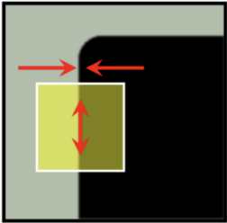
Consider a simplified image where background pixels have an intensity value of 128 (gray) and object pixels have a value of 0 (black). Let's trace how the Moravec detector evaluates a candidate pixel step-by-step:

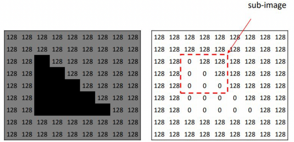
1. Selecting the Reference Sub-Image

The detector places a small sliding window $W$ (e.g., $2 \times 2$) centered at the candidate pixel location $(m,n)$ to capture the local intensity structure:

Original Window $W$ at $(m,n)$: $I(m,n) = 0$ $I(m,n+1) = 128$ $I(m+1,n) = 128$ $I(m+1,n+1) = 128$

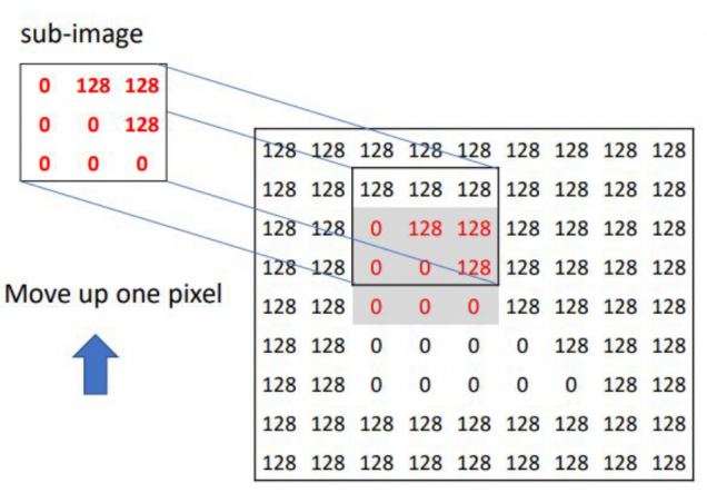
2. Shift Up by One Pixel: $(x,y) = (0, -1)$

The sub-image is shifted one pixel upward and compared with the original window to evaluate intensity variation.

Shifted Window at $(m, n-1)$: $I(m, n-1) = 128$ $I(m, n) = 0$ $I(m+1, n-1) = 128$ $I(m+1, n) = 128$ \[\text{SSD} = (0 - 128)^2 + (128 - 0)^2 + (128 - 128)^2 + (128 - 128)^2\] \[\text{SSD} = 16384 + 16384 + 0 + 0 = 32768 \quad (\text{Large!})\]

A large SSD value indicates strong intensity variation when shifting upward, contributing evidence toward detecting a corner.

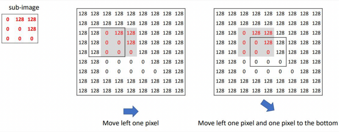
3. Horizontal, Vertical, and Diagonal Shifts

The process is repeated for shifts in other directions. Suppose we shift right:

Shifted Window at $(m, n+1)$ (Right shift): $I(m, n+1) = 128$ $I(m, n+2) = 128$ $I(m+1, n+1) = 128$ $I(m+1, n+2) = 128$ \[\text{SSD} = (0 - 128)^2 + (128 - 128)^2 + (128 - 128)^2 + (128 - 128)^2\] \[\text{SSD} = 16384 + 0 + 0 + 0 = 16384 \quad (\text{Large!})\]

If the window is shifted in a direction that aligns perfectly with an edge (e.g., shifting parallel to an edge), the pixel intensities will not change, resulting in a small SSD. Only when the intensity variation remains large for all tested shifts (meaning the minimum SSD $F_{m,n}$ is still high) is the pixel classified as a corner.