Lecture 6: Image Analysis

Why pyramids?

Multi-scale object search problem

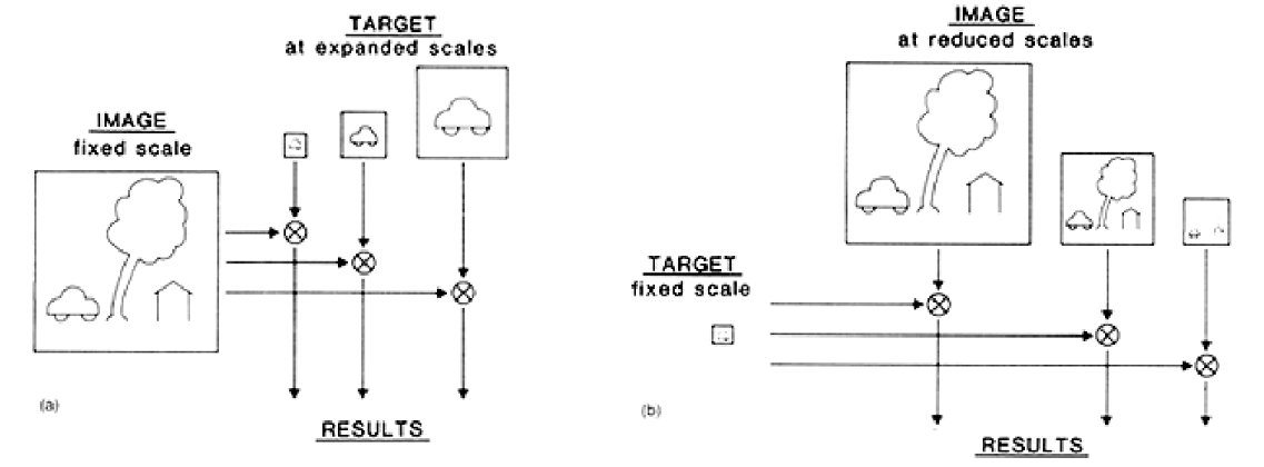
Suppose we want to detect a bird in an image using a small bird template. Because the bird may appear at different scales depending on its distance from the camera, a single-scale template match will fail.

Two Main Approaches to Multi-Scale Search:
1. Scale the target image: Perform template matching against multiple progressively scaled versions of the target scene.
2. Scale the template image: Compare multiple resized versions of the template against the original, high-resolution target image.

Image pyramids allow us to perform these searches efficiently by organizing representation scale-by-scale.

Pyramid structure

G₄

Level 4 (top) — smallest, lowest resolution. (M/16)×(N/16)

G₃

Level 3 — (M/8)×(N/8)

G₂

Level 2 — (M/4)×(N/4) — ¼ pixels of level below

G₁

Level 1 — (M/2)×(N/2)

G₀

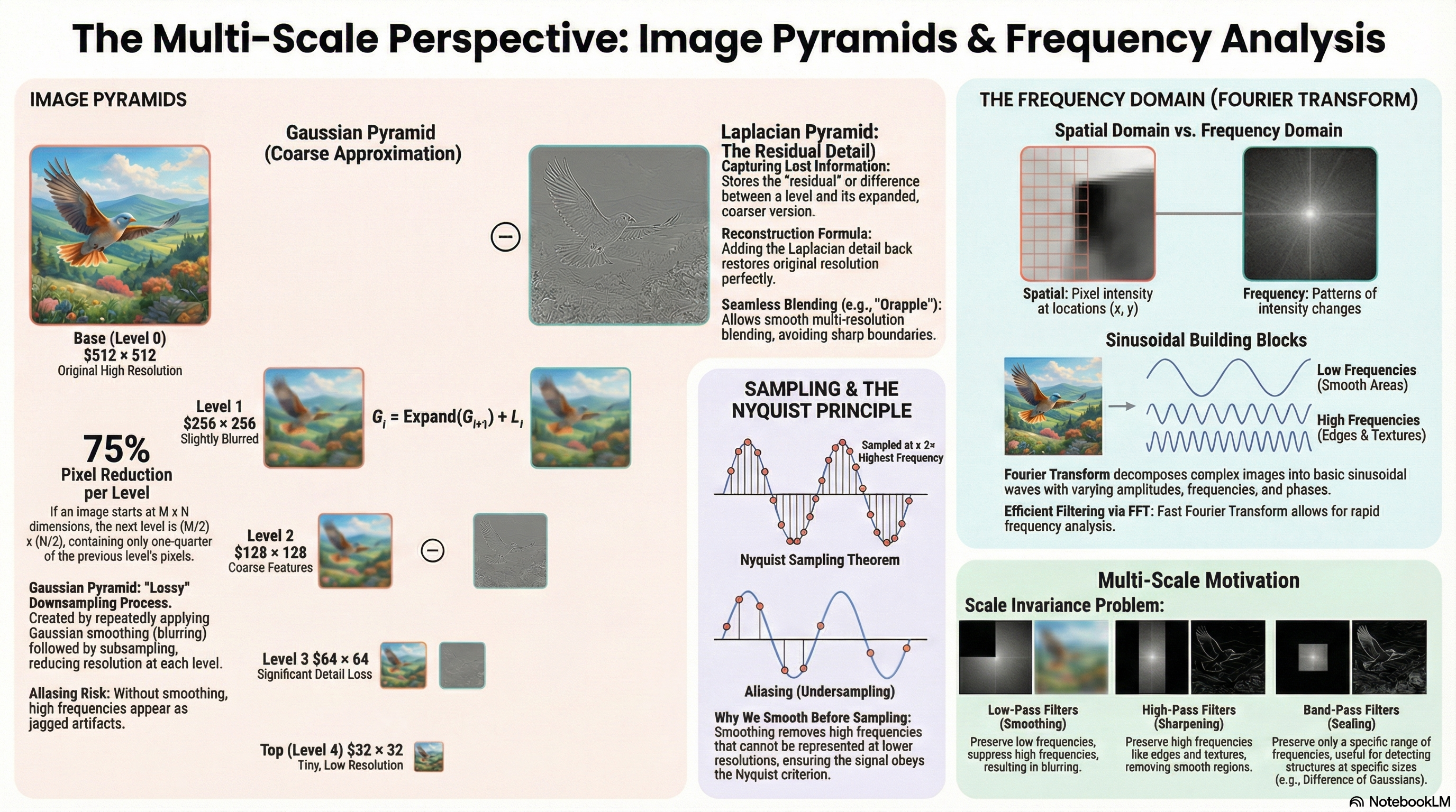
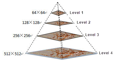
Level 0 (base) — original image M×N. Highest resolution.

Key storage fact: Each level has ¼ the pixels of the level below (halved in both dimensions). A full pyramid takes only 4/3 × the original storage (geometric series sum: $1 + 1/4 + 1/16 + ... = 4/3 \approx 1.333$).

Two fundamental pyramid operations

Reduce (going UP the pyramid)

1. Gaussian smooth (low-pass filter) to remove high frequencies.

2. Subsample by a factor of 2 (take every 2nd row and column).

Result: half the width and height.

Must smooth BEFORE subsampling to prevent aliasing artifacts.

Expand (going DOWN the pyramid)

1. Double the width and height (upsample).

2. Insert zeros between known pixel values.

3. Apply an interpolating low-pass filter to estimate missing values.

Result: coarser approximation at twice the resolution.

Gaussian pyramid — construction

Algorithm: 1. Start with original image G₀ 2. Apply Gaussian blur to G_l 3. Subsample every 2nd row and column → G_{l+1} 4. Repeat until minimum resolution reached Properties: • Each level is a blurred, downsampled version of the level below • Higher levels = coarser / lower resolution • Lossy — smoothing discards high-freq detail permanently

Gaussian vs Laplacian pyramid — quick compare

Gaussian pyramid

Stores smoothed + downsampled images

Compact multi-scale representation

Lossy — cannot reconstruct original exactly

Gives coarse approximation at each scale

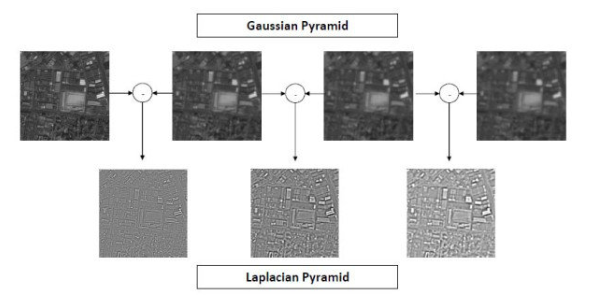
Laplacian pyramid

Stores DIFFERENCE between Gaussian levels

Captures fine detail lost during smoothing

Lossless — exact reconstruction possible

Gives residual / detail at each scale

The core question Laplacian pyramids solve

Can we reconstruct the original image from a Gaussian pyramid?

NO. Smoothing permanently discards fine edges, textures, and sharp transitions. The Laplacian pyramid solves this by storing what was lost at each level as a residual image.

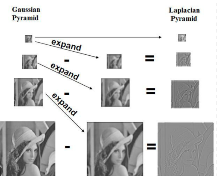
Construction — storing the lost detail

Algorithm: 1. Build the Gaussian pyramid: $G_0, G_1, G_2, \dots, G_n$ 2. For each level $l = 0, 1, \dots, n-1$: a. Expand $G_{l+1}$ to the size of $G_l$: $\text{Expand}(G_{l+1})$ b. Compute the difference: $L_l = G_l - \text{Expand}(G_{l+1})$ c. Store the residual image $L_l$ 3. Keep the smallest Gaussian image $G_n$ as the top of the pyramid. Full Laplacian Pyramid representation: $\{L_0, L_1, L_2, \dots, L_{n-1}, G_n\}$ Where $L_l$ contains the fine spatial details (edges, textures, sharp transitions) present in $G_l$ but missing from the coarser level.

What Laplacian images look like: Edge-like, detail-emphasizing images. Smooth regions → near-zero values. Edges and textures → non-zero values. They look like embossed versions of the original.

Reconstruction — adding back the detail

Reconstruction Equation: $G_l = \text{Expand}(G_{l+1}) + L_l$ Algorithm (Bottom-Up Reconstruction): 1. Start from the smallest Gaussian image $G_n$ (the top of the pyramid). 2. For each level $l$ from $n-1$ down to $0$: a. Expand the Gaussian image at level $l+1$: $\text{Expand}(G_{l+1})$ b. Add the residual at level $l$: $L_l$ c. Reconstruct the Gaussian image at level $l$: $G_l = \text{Expand}(G_{l+1}) + L_l$ 3. After $n$ steps, recover $G_0$, which is exactly the original image (lossless!).

Connection to DoG

Laplacian pyramid ≈ Difference of Gaussians (DoG)

L_l = G_l − Expand(G_{l+1}) is structurally equivalent to subtracting two Gaussian-smoothed versions at different scales: DoG = G_σ₁ − G_σ₂ where σ₂ > σ₁. Both suppress slowly varying content and emphasize structures that change rapidly (edges, blobs). DoG is used in SIFT for this reason.

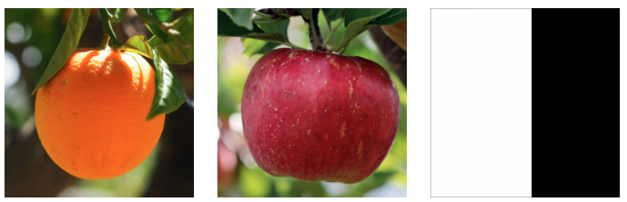
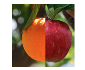
Laplacian pyramid blending — the apple/orange example

Direct Combination (Sharp Seam)

Combine images directly using a binary mask.

Result: A sharp, highly visible boundary seam.

Unnatural transition: The cut happens abruptly at one pixel location, highlighting contrast and color differences.

Multi-Resolution Blending (Pyramid)

Decompose images into Laplacian pyramids.

Convert mask to Gaussian pyramid (softens seam at lower scales).

Natural transition: Blend level-by-level, then reconstruct the final image.

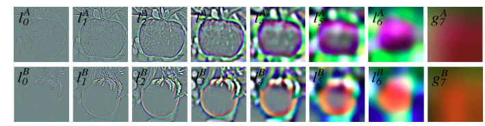
Build Laplacian pyramids for BOTH images (apple and orange).

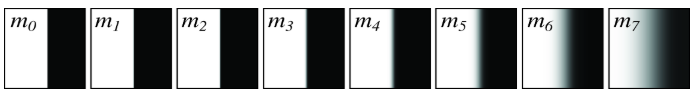
Build a Gaussian pyramid of the binary mask (mask gets smoother and transition zone becomes wider at coarser levels).

At each level $l$, blend Laplacian levels using the matching mask level: $B_l = mask_l \cdot LA_l + (1 - mask_l) \cdot LB_l$.

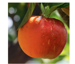
Reconstruct the blended pyramid bottom-up to obtain the final seamlessly blended image.

Why pyramid blending works: Low-frequency (coarse) detail is blended over a wide transition zone. High-frequency (fine) detail is blended over a narrow zone. Each scale gets the right amount of blending — no ghosting, no harsh seam.

Uses of Laplacian pyramid

Image compression

Residuals often sparse — encode efficiently

Image blending

Scale-aware seamless compositing

Multi-scale detection

Find structures at different sizes

Denoising

Separate noise from detail by scale

Image fusion

Focus stacking, HDR merging

Feature extraction

Scale-space analysis

What is aliasing?

Sampling too slowly to represent the signal accurately

High-frequency components can't be captured at the lower sampling rate. They "fold back" and appear as incorrect lower-frequency patterns. Result: jagged edges, false patterns, moiré, pixelated textures.

Nyquist sampling theorem

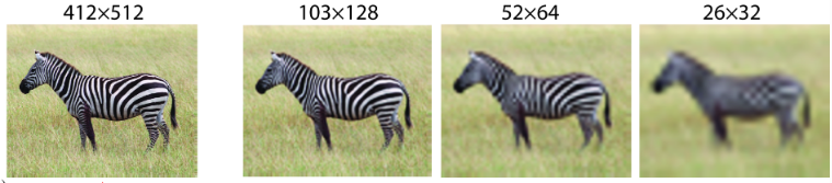
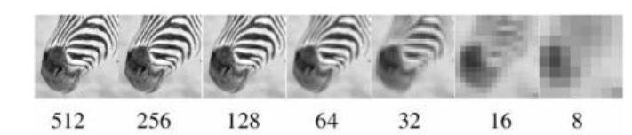
Nyquist Criterion: $f_{\text{sampling}} \ge 2 \times f_{\text{max\_signal}}$ To represent a repeating spatial pattern: We need at least 2 samples (pixels) per cycle/period of the pattern. Case Study: Downsampling Zebra Stripes (High Spatial Frequencies) The zebra stripes contain high spatial frequencies because the intensity changes rapidly between black and white. Let's trace how the pattern behaves as we decrease resolution (sample too slowly): • 512, 256, and 128 pixels: There are enough pixels/samples to represent the stripe details clearly. • 64 and 32 pixels: The number of pixels becomes smaller, causing the fine stripe patterns to weaken. • 16 and 8 pixels: The image no longer has enough samples to represent the stripe pattern correctly, violating the Nyquist criterion. The stripes are lost or distorted, producing aliasing (false lower-frequency patterns, Moiré effects, and pixelated textures).

The rule: You must sample at least TWICE the highest frequency in the signal. If you can't sample fast enough, remove the high frequencies FIRST (low-pass filter), then sample. This is exactly what the Gaussian pyramid does.

Why you MUST smooth before subsampling

Subsample without smoothing

High-freq content still in image

Nyquist violated at lower resolution

High freqs appear as false low-freq patterns

Jagged edges, moiré artifacts

Smooth THEN subsample (correct)

Gaussian removes freqs above new Nyquist limit

Remaining content representable at lower res

No aliasing artifacts

Visually stable reduction

Anti-aliasing strategies

Oversampling

Increase the sampling rate

Preserve high-frequency information

Cost: more data, more compute

Used in: supersampling anti-aliasing (SSAA)

Low-pass filtering (practical)

Apply Gaussian before downsampling

Removes problematic high freqs

Some information lost — but stable

Standard approach in image pyramids

Aliasing in real applications

Scenario	What happens	Solution
Image downsampling	Fine textures become moiré patterns	Gaussian blur first
Video frame rate	Wagon wheels appear to spin backward	Higher frame rate (oversample)
3D texture mapping	Shimmering distant surfaces	Mipmapping (pyramid)

Spatial vs frequency domain

Spatial domain

Image = grid of pixel intensities

Each value = brightness at location (x,y)

Filtering = sliding kernel over pixels

Frequency domain

Image = collection of sinusoidal patterns

Each component = frequency + amplitude + phase

Filtering = multiply/zero frequency components

Sinusoidal building block

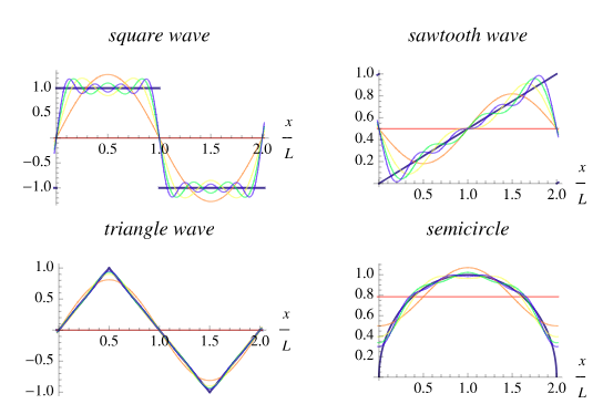
Fundamental Sinusoidal Signal: \[f(x) = A \cdot \sin(\omega x + \phi)\] Where: • $A$: Amplitude (strength or maximum height of the wave) • $\omega$: Frequency of oscillation (how fast the wave repeats/oscillates) • $x$: Spatial or temporal variable (position or time coordinate) • $\phi$: Phase shift (where the wave cycle starts relative to the origin) Fourier Principle: Any complex signal can be decomposed into and reconstructed by combining a sum of sinusoidal waves with different amplitudes, frequencies, and phase shifts. This is computed using the Fourier Transform.

Physical/Spatial Meaning of Nyquist: In digital image processing, a spatial frequency pattern with a period (wavelength) of $T$ pixels (e.g., repeating black and white stripes every $T$ pixels) requires at least 2 pixels per period (i.e. sample spacing $\le T/2$) to be faithfully captured without aliasing.

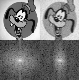
Frequency interpretation in images

Low frequencies

Slow, gradual intensity changes

Smooth regions, background

Overall shape and illumination

Center of Fourier spectrum

High frequencies

Rapid intensity changes

Edges, textures, fine detail

Noise often lives here

Periphery of Fourier spectrum

DFT and FFT

Discrete Fourier Transform (DFT)

Decomposes a discrete (pixel) image into frequency components. Each output F(u,v) tells us the amplitude and phase of a particular 2D sinusoidal pattern in the image. The FFT (Fast Fourier Transform) computes the DFT efficiently — O(N log N) instead of O(N²).

Fourier Spectrum Characteristics & Effects

Fourier Spectrum Edge Effects

The Phenomenon: A prominent vertical line frequently appears in the Fourier spectrum of real images.

The Cause: Caused by edge effects (artifacts resulting from boundary discontinuities between the opposite edges of the image when treated as periodic).

Horizontal Smoothing Effect

The Phenomenon: Horizontal smoothing reduces high-frequency components in the horizontal direction.

The Cause: Smoothing removes rapid intensity changes, effectively cutting off high spatial frequencies in the direction of the blur.

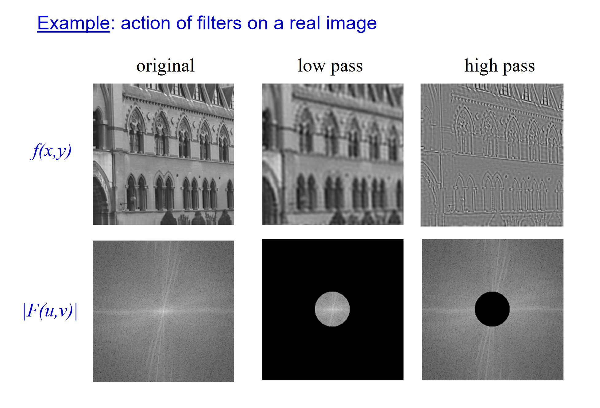
Frequency domain filters — full comparison

Low-pass filter

Keeps: Low frequencies (center)

Removes: High frequencies (edges)

Effect: Blurring / smoothing

Example: Gaussian filter

High-pass filter

Keeps: High frequencies (edges)

Removes: Low frequencies (center)

Effect: Edge / detail enhancement

Example: Sobel, Laplacian

Band-pass filter

Keeps: A range of frequencies

Removes: Very low and very high

Effect: Texture detection at scale

Example: DoG

Convolution theorem — the key link

Convolution theorem: Spatial convolution ↔ Frequency multiplication f ⋆ g ←→ F(u,v) · G(u,v) Steps for frequency-domain filtering: 1. Compute FFT of image: F = FFT(image) 2. Compute FFT of kernel: H = FFT(kernel) 3. Multiply: Result = F · H (element-wise) 4. Compute inverse FFT: filtered_image = IFFT(Result) Practical advantage: for LARGE kernels, frequency-domain multiplication is FASTER than spatial convolution.

Why this matters: The convolution theorem tells us that spatial filtering (sliding kernel) and frequency filtering (multiplying spectra) are equivalent. A Gaussian low-pass filter in spatial domain = circle mask in frequency domain zeroing high-frequency components.

Spatial ↔ frequency filter equivalences

Spatial domain filter	Frequency domain equivalent	Effect
Gaussian blur	Low-pass (smooth circle in center)	Smoothing
Sobel / Laplacian	High-pass (ring at periphery)	Edge enhancement
DoG	Band-pass (annular ring)	Texture / blob detection