Lecture 5: Image Filtering

What is filtering?

Image → new image via local or global rules

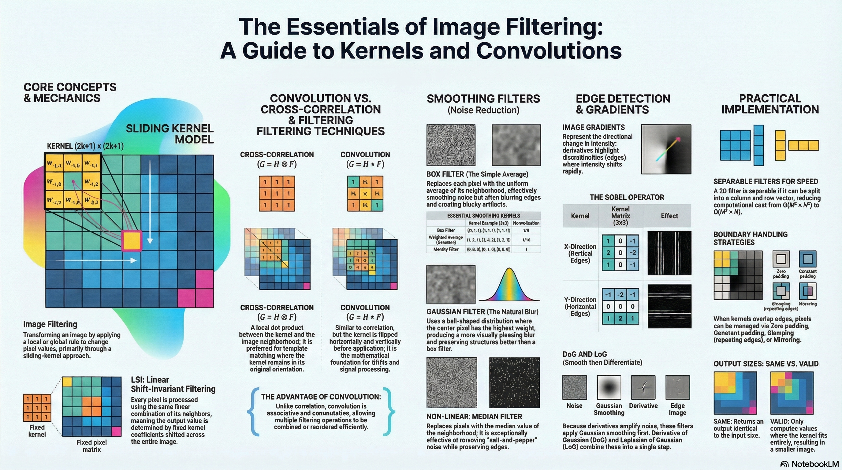
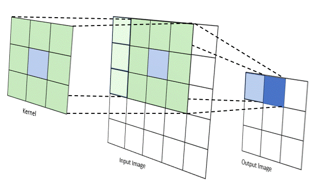
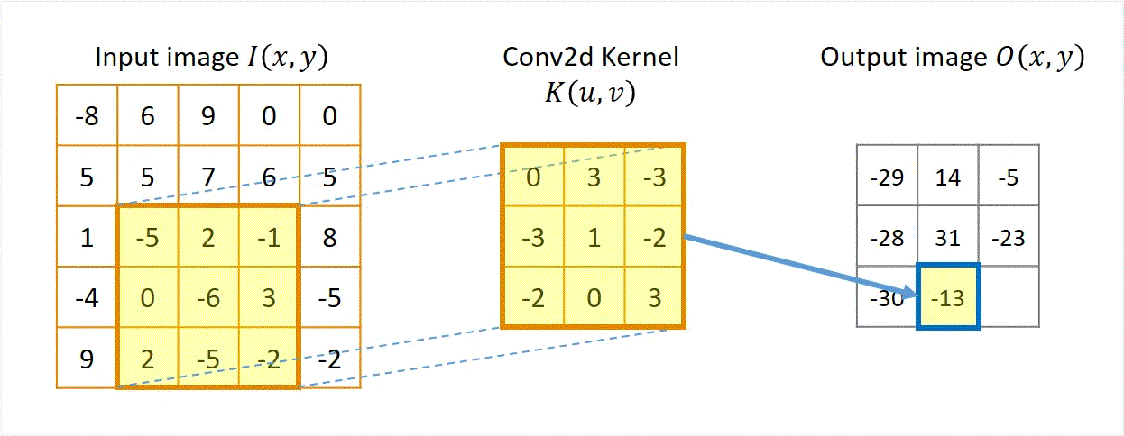
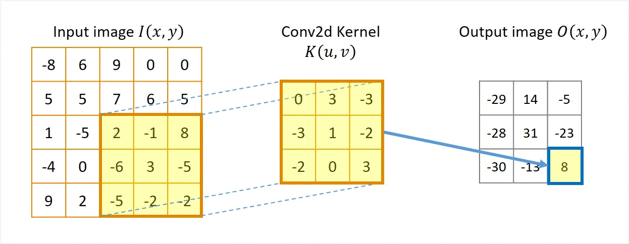
Two approaches: Sliding-kernel (kernel moves over every pixel — the main focus) and segmentation-based (partition into regions first). Sliding-kernel is the foundation of classical methods AND CNNs.

LSI filtering — the core model

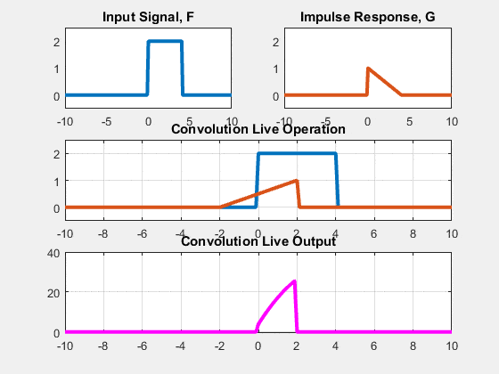
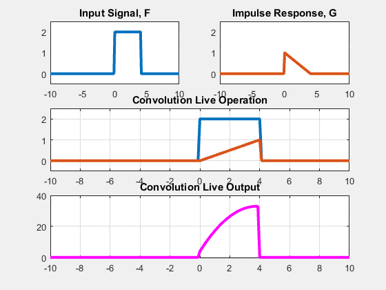
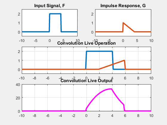
g[m,n] = Σ_(k,l) h[k,l] · f[m+k, n+l] f = input image h = kernel (filter weights) g = output image Linear: output is weighted sum of neighbors Shift-invariant: same kernel applied at EVERY pixel location

Why CNNs matter here: Convolutional layers in CNNs ARE learned LSI filters. Understanding kernel sliding is the basis for understanding CNNs.

Kernel size convention: (2k+1) × (2k+1)

k=1 → 3×3

1 pixel radius. 9 neighbors.

k=2 → 5×5

2 pixel radius. 25 neighbors.

k=3 → 7×7

3 pixel radius. 49 neighbors.

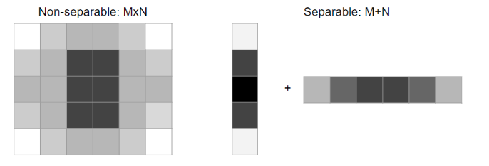
Separable filters — computational efficiency

A 2D filter is separable if it can be factored as the outer product of a column vector and a row vector.

Instead of performing a full 2D convolution, we can split it into two consecutive 1D convolutions: convolve vertically with the column filter, then convolve the result horizontally with the row filter.

Factoring Equation: H = v · wᵀ (where v is a column vector N×1, and wᵀ is a row vector 1×N) 2D Convolution Separation (Associativity): G = H ⋆ F = (v · wᵀ) ⋆ F = v ⋆ (wᵀ ⋆ F) Computational Complexity: Non-separable cost: O(M² × N²) — N² multiplications per pixel Separable cost: O(M² × 2N) — 2N multiplications per pixel Example (N = 15 kernel): Non-separable: 225 multiplications/pixel Separable: 30 multiplications/pixel (7.5× computational speedup!)

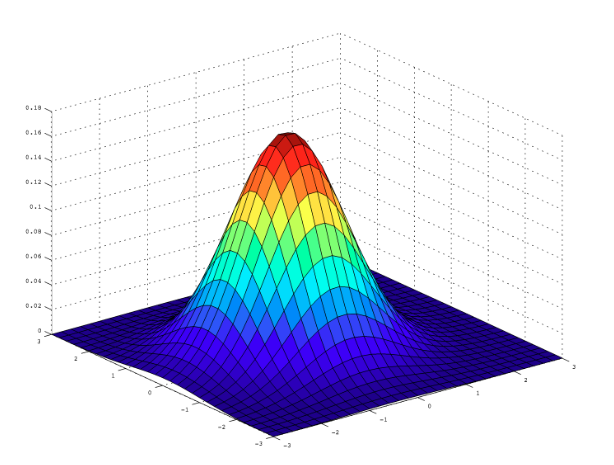
Gaussian Filters: 2D Gaussian kernels are mathematically separable, which makes them highly efficient to compute even for large standard deviations.

Boundary handling options

Strategy	What it does	Pros & Cons (Use when)
Zero padding	Outside pixels are set to 0	Simple, but introduces dark border artifacts as the black boundary pulls down intensity values during averaging.
Clamp/replicate	Repeat the nearest edge pixel values outward	Avoids dark border artifacts by extending the border intensity value. Good default.
Mirror/reflect	Reflect pixels symmetrically across the boundary	Creates a smooth, continuous transition without discontinuities at the boundary. Preferred for derivative filters.
Wrap/toroidal	Loop image coordinates around (left connects to right)	Assumes periodic signals. Ideal for Fourier/frequency-domain analysis.

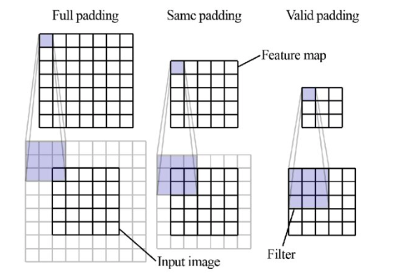
Output size modes

Full

All overlaps including beyond edges

Larger than input

Same

Output = same size as input

Requires padding

Valid

Kernel fully inside image only

Smaller than input

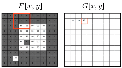
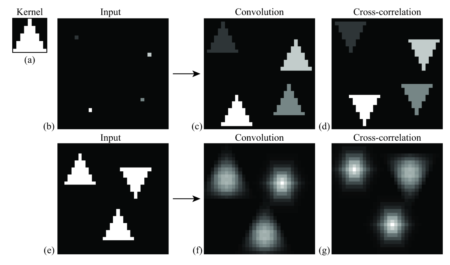
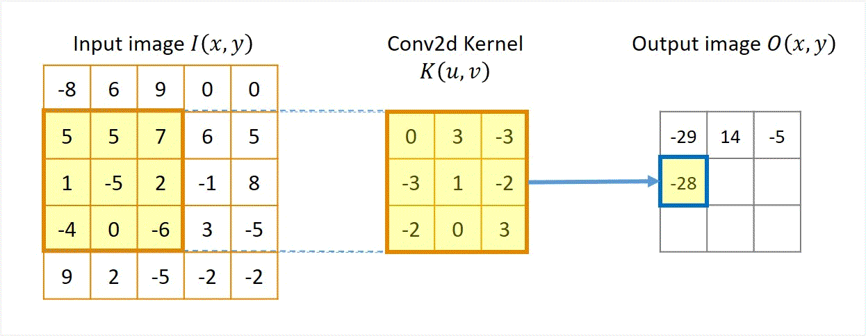
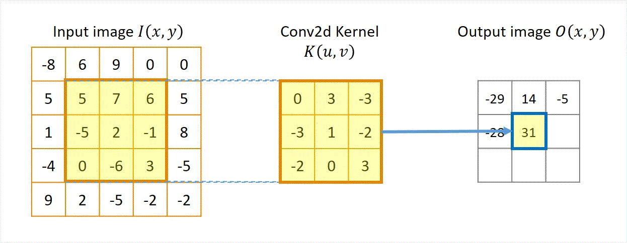
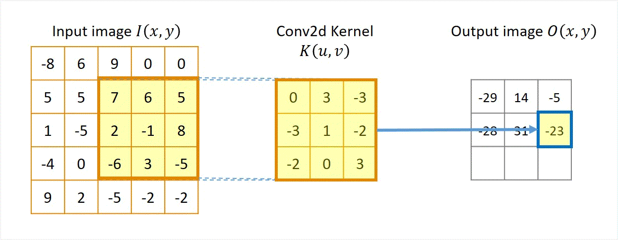
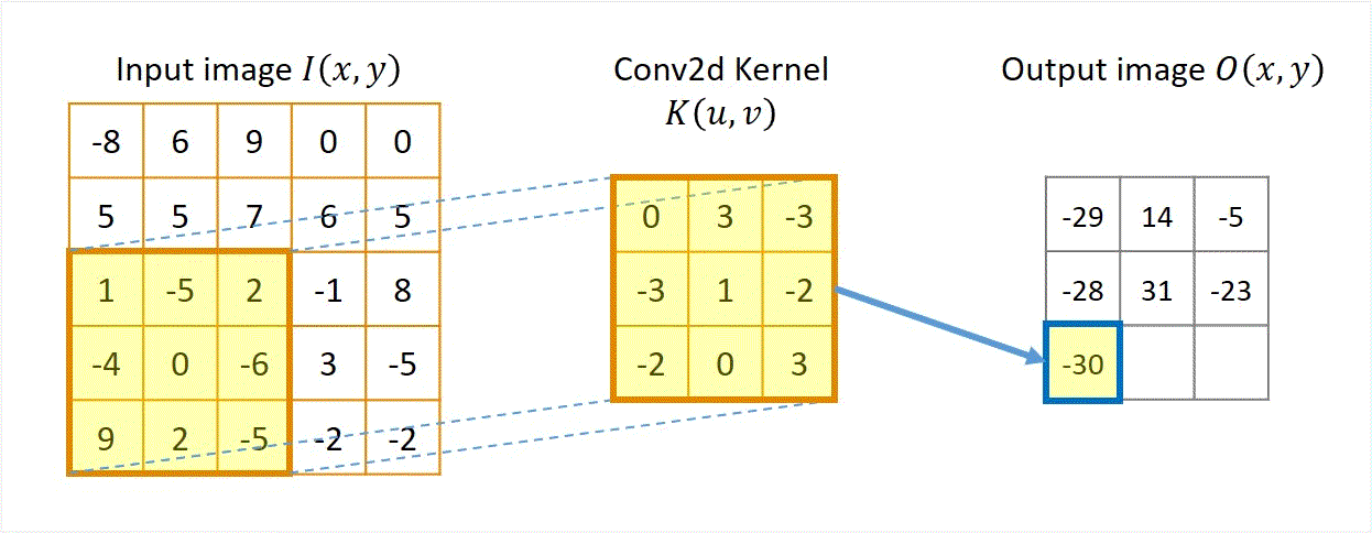
Cross-correlation

G[i,j] = Σ_(u=−k to k) Σ_(v=−k to k) H[u,v] · F[i+u, j+v] Compact: G = H ⊗ F Where: (i, j) = target output pixel coordinate in the image (u, v) = relative kernel coordinate from the center H[u, v] = kernel coefficient at index (u, v) F[i+u, j+v] = neighboring pixel value in original image

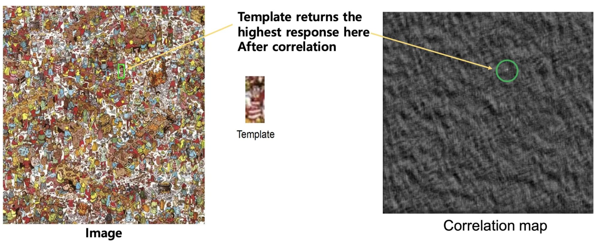
Key Property & Use Case

The kernel is used in its original orientation. The output responds strongly at coordinates where the local image region matches the kernel pattern. Ideal for template matching and similarity measurement.

Convolution

G[i,j] = Σ_(u=−k to k) Σ_(v=−k to k) H[u,v] · F[i−u, j−v] Compact: G = H ⋆ F Kernel flipping behavior: H_flipped[u, v] = H[−u, −v] (mirrored horizontally and vertically)

Key Property & Use Case

The kernel is flipped 180° (both rows and columns reversed) before computing the dot product. This is the standard operator in signal processing, filter analysis, and CNN layers.

Kernel flipping — the only difference

Original kernel

Flipped kernel (for convolution)

When are they identical? When the kernel is symmetric (rotationally symmetric around the center) — e.g. Gaussian, box filter, Laplacian. For asymmetric kernels (e.g. Sobel, directional edge filters) convolution and correlation produce different outputs.

Why convolution matters more (algebraic properties)

Cross-correlation properties

Does NOT support associativity.

Does NOT support commutativity.

Matching is intuitive but mathematically less convenient for chaining.

Convolution properties

Commutative: f ⋆ h = h ⋆ f

Associative: (f ⋆ h₁) ⋆ h₂ = f ⋆ (h₁ ⋆ h₂)

Distributive: f ⋆ (h₁ + h₂) = (f ⋆ h₁) + (f ⋆ h₂)

Associativity Example: Apply Gaussian blur then derivative: (G ⋆ I) derivative = (∂G/∂x) ⋆ I This allows pre-combining multiple filters into a single combined kernel. DoG (Difference of Gaussians) is a direct practical application of this.

Special kernel behaviors

Identity kernel

Output = exact copy of input

Shift left kernel

Output = input shifted left by 1px

Sharpening kernel

−⅑

+⁸⁄₉

−⅑

2×identity − box. Enhances edges.

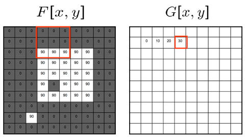
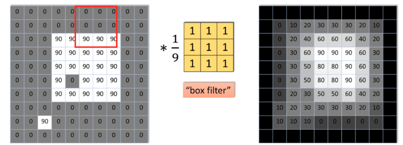
Box filter (mean/average)

3×3 box kernel (×1/9)

Box filter properties

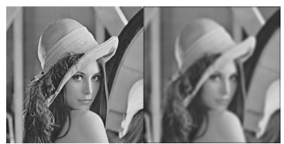
All weights inside the kernel window are equal (uniform averaging).

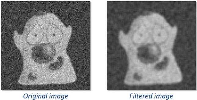
Blurs noise but also strongly blurs sharp structural edges.

Frequency response has a sharp cut-off, causing blocky artifacts.

Kernel is scaled by 1/(kernel area) so weights sum to exactly 1.

Gaussian filter

3×3 Gaussian kernel (×1/16)

Gaussian filter properties

Center pixel receives largest weight; decay follows 2D normal curve.

Separable → vertically then horizontally convolved.

Symmetric and isotropic: smooth blur with no blocky artifacts.

σ controls the spatial spread (wider window needed for large σ).

Standard Gaussian Kernel Matrices

5×5 Gaussian (÷273)

1 4 7 4 1
4 16 26 16 4
7 26 41 26 7
4 16 26 16 4
1 4 7 4 1

7×7 Gaussian (÷1003)

0 0 1 2 1 0 0
0 3 13 22 13 3 0
1 13 59 97 59 13 1
2 22 97 159 97 22 2
1 13 59 97 59 13 1
0 3 13 22 13 3 0
0 0 1 2 1 0 0

Impulse Response: Box vs. Gaussian

What is an impulse response?

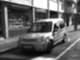
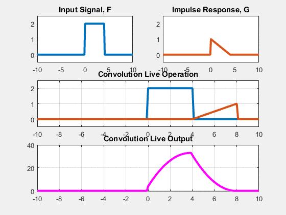
The impulse response is the output produced by the filter when the input is a single isolated bright pixel (analogous to a Dirac delta in continuous signals).

Box filter response: Spreads the energy uniformly inside a finite square window. It has a sharp spatial cut-off, causing blocky, unnatural ringing artifacts.

Gaussian filter response: Spreads the energy smoothly. The weights decay gradually with distance from the center, producing a natural-looking blur and fewer artifacts. This makes it far more stable as a pre-smoothing filter before gradient edge extraction.

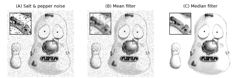
Non-linear filters

Median filter

Sort neighborhood pixel values, take the median.

Excellent for salt-and-pepper / impulse noise.

Outlier pixels are completely ignored by the median sorting.

Preserves sharp edges better than linear mean filters.

Strictly non-linear: output is not a weighted sum.

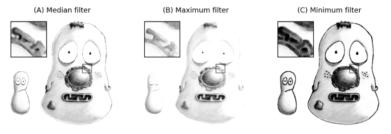
Dilation (max filter)

Replace center pixel with neighborhood MAX.

Expands and grows bright regions in the image.

Core operator of mathematical morphology.

Used for shape-based structural processing.

Erosion (min filter)

Replace center pixel with neighborhood MIN.

Shrinks and erodes bright regions.

Core operator of mathematical morphology.

Used for shape-based structural processing.

Median vs Gaussian noise handling: Gaussian filters are best for general additive Gaussian noise. Median filters are specifically designed for salt-and-pepper / impulse noise where outliers are extreme (0 and 255). A mean filter would average the outlier in, blurring the corruption across the entire window, whereas a median filter completely rejects it.

Noise types and best filter

Noise type	Description	Best filter
Gaussian noise	Normal-distributed intensity variation	Gaussian / box filter
Salt-and-pepper	Random black and white pixels	Median filter
Impulse noise	Random bright (white) pixels only	Median filter

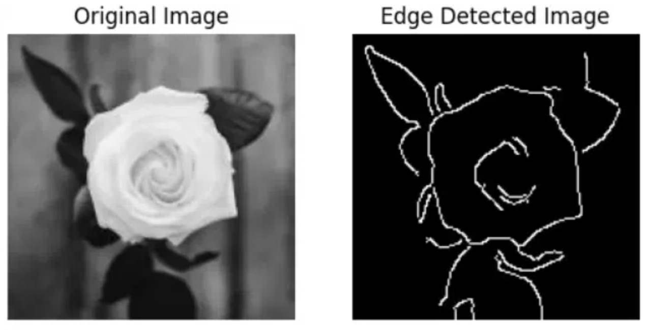
Why derivatives detect edges

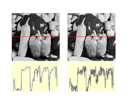
Edges correspond to sudden, rapid changes in image intensity. In mathematical terms, edges represent discontinuities, which can be highlighted by computing spatial derivatives (gradients), as derivatives become very large at these transitions.

1D discrete derivative example: Array values: [10, 200, 210] at positions f(x−1), f(x), f(x+1) Approximate Central Derivative at f(x): f'(x) = ( f(x+1) − f(x−1) ) / 2 = ( 210 − 10 ) / 2 = 100 ← strong numerical response indicating an edge

Discrete Differentiation is Sensitive to Noise: Even tiny random intensity fluctuations (noise) produce large derivative spikes. To prevent this, the standard pipeline is: SMOOTH first, then DIFFERENTIATE. Pre-smoothing with a Gaussian filter suppresses noise before gradient calculation.

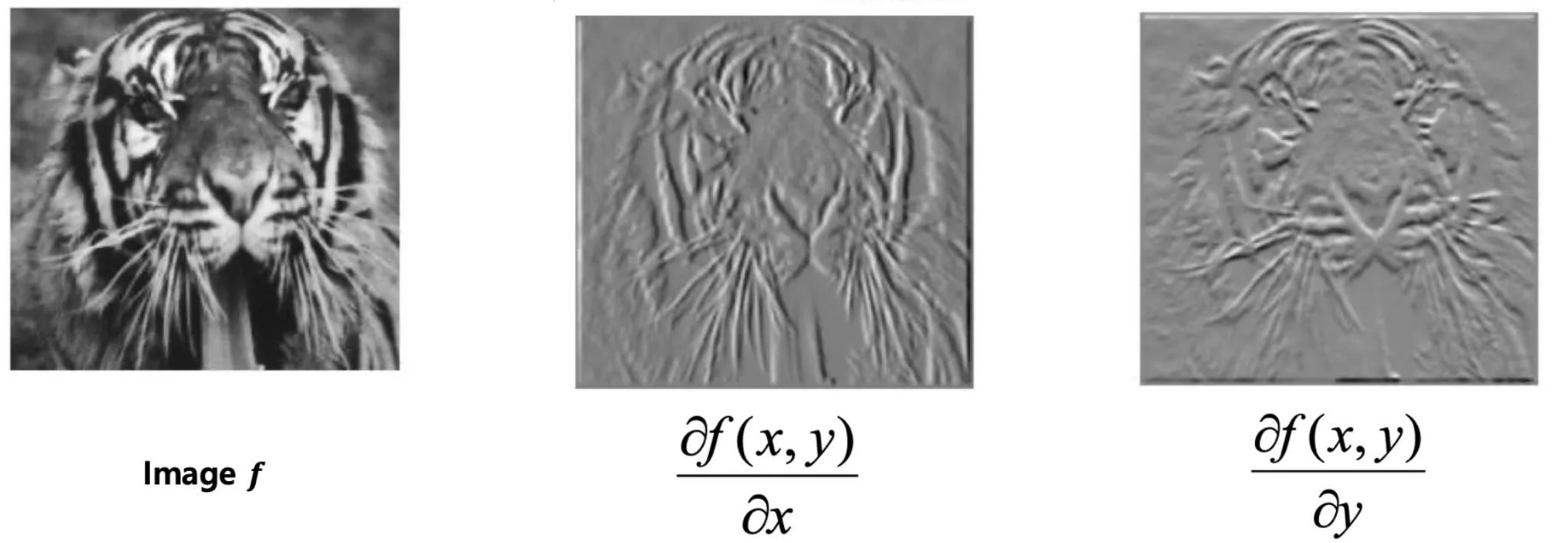
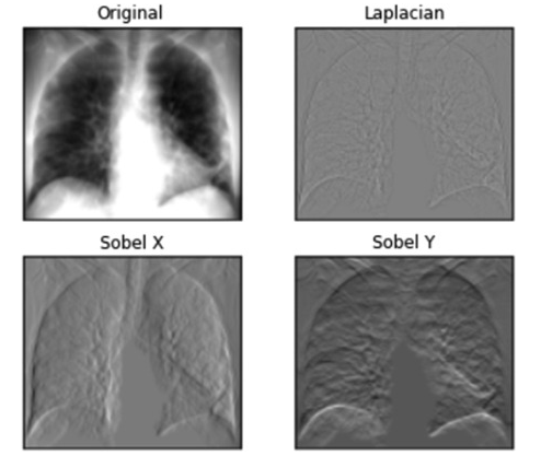
Why derivative images look "embossed"

The derivative measures the directional change of intensity. Smooth regions with little change appear grey/neutral. Edges produce bright positive responses (transitioning from dark to bright) or dark negative responses (transitioning from bright to dark). This highlights boundaries like raised reliefs, giving the output an embossed appearance.

Sobel filter — directional first derivative

Smoothing + Differentiation Combined

The Sobel filter computes the directional gradient at each pixel while incorporating smoothing in the orthogonal direction to improve stability against noise.

CRITICAL EXAM CONCEPT: Direction of Detection vs. Direction of Edge
• The horizontal gradient kernel $G_x$ detects changes in the horizontal direction ($x$), which means it detects vertical edges (left-right transitions).
• The vertical gradient kernel $G_y$ detects changes in the vertical direction ($y$), which means it detects horizontal edges (top-bottom transitions).

Horizontal Gradient Gₓ (Vertical Edges)

−1

−2

−1

Vertical Gradient G_y (Horizontal Edges)

−1

−2

−1

Why the 2s in Sobel?

Each kernel is a convolution of a derivative and a smoothing vector:

Horizontal smoothing: [1, 2, 1]ᵀ (Gaussian approximation)

Vertical derivative: [1, 0, −1]

Saves cost: Both kernels are separable.

Gradient Magnitude: |G| = √(Gₓ² + G_y²) (often approximated as |Gₓ| + |G_y|) Gradient Direction (Angle): θ = tan⁻¹( G_y / Gₓ )

DoG vs LoG — combining smooth + detect

Derivative of Gaussian (DoG)

First derivative operator.

∂/∂x(G ⋆ I) = (∂G/∂x) ⋆ I

Convolve image directly with the derivative of a Gaussian kernel.

Saves one filtering pass via associativity.

Responds strongly to directional edges.

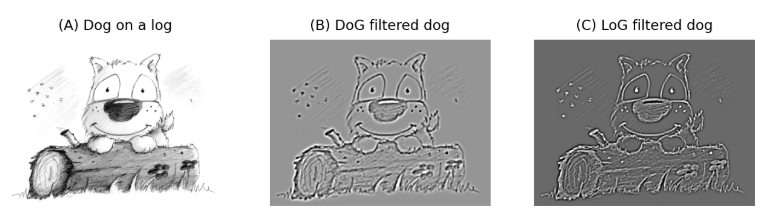
Laplacian of Gaussian (LoG)

Second derivative operator.

∇²(G ⋆ I) = (∇²G) ⋆ I

Convolve image directly with the second spatial derivative (Laplacian) of a Gaussian.

Isotropic: responds equally to transitions in all directions.

Best for edge detection and blob detection.

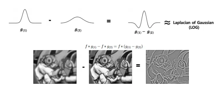
DoG as approximation to LoG

Difference of Gaussians (DoG) ≈ LoG

Subtracting two Gaussian-blurred versions of an image at different scales ($\sigma_1$ and $\sigma_2$) closely approximates the second derivative of the Laplacian of Gaussian:

DoG = G(σ₁) − G(σ₂) (where σ₁ ≠ σ₂)

This is highly preferred in practice because subtracting two blurred images is computationally much faster than computing a full LoG kernel. It is a core step in keypoint detection for SIFT (Scale-Invariant Feature Transform).

Edge detection filter comparison

Filter	Derivative order	Direction	Noise handling	Best for
Sobel	1st	X or Y (directional)	Built-in smoothing orthogonal to derivative	Edge direction, gradient magnitude maps
DoG	1st	Directional derivative	Sizable Gaussian pre-smoothing	Scale-space edges, SIFT descriptor keypoints
LoG	2nd	All directions (isotropic)	Sizable Gaussian pre-smoothing	Isotropic edge extraction, blob detection

Key pipeline reminder: Derivatives amplify noise. Always apply Gaussian smoothing before taking derivatives, or combine both into a single step convolving with derivative-of-Gaussian or Laplacian-of-Gaussian kernels to preserve computational efficiency.

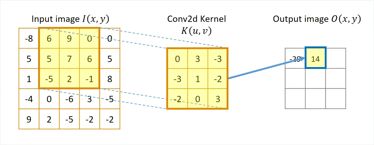
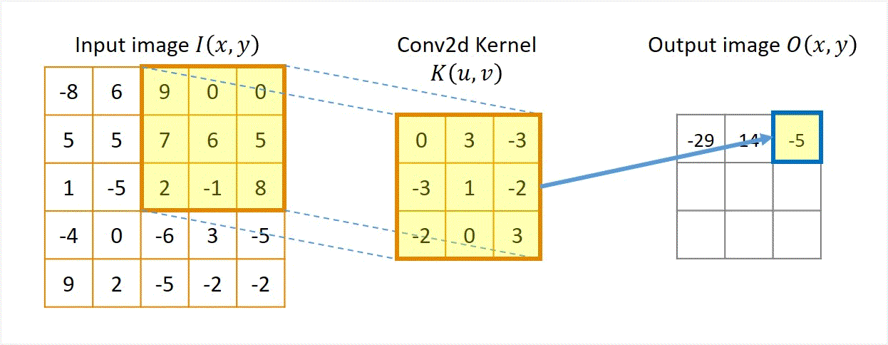
Convolution step-by-step calculator

Enter a 5×5 image patch and a 3×3 kernel. Computes the correlation output at the center pixel.

Image patch (5×5) — center pixel is highlighted

Kernel (3×3) — select preset or edit values

Separability cost calculator

Image size M×M1000

Kernel size N×N15

Sobel gradient magnitude demo

Enter 3×3 image patch. Computes Gₓ, G_y, and gradient magnitude at center pixel.