Lecture 4: Image Enhancement

General Enhancement Operator

g(x) = T( f(x) ) Where: f(x) = input image signal at pixel location x T = transformation operator (point mapping or neighborhood rule) g(x) = output transformed image signal

Organizing Principle

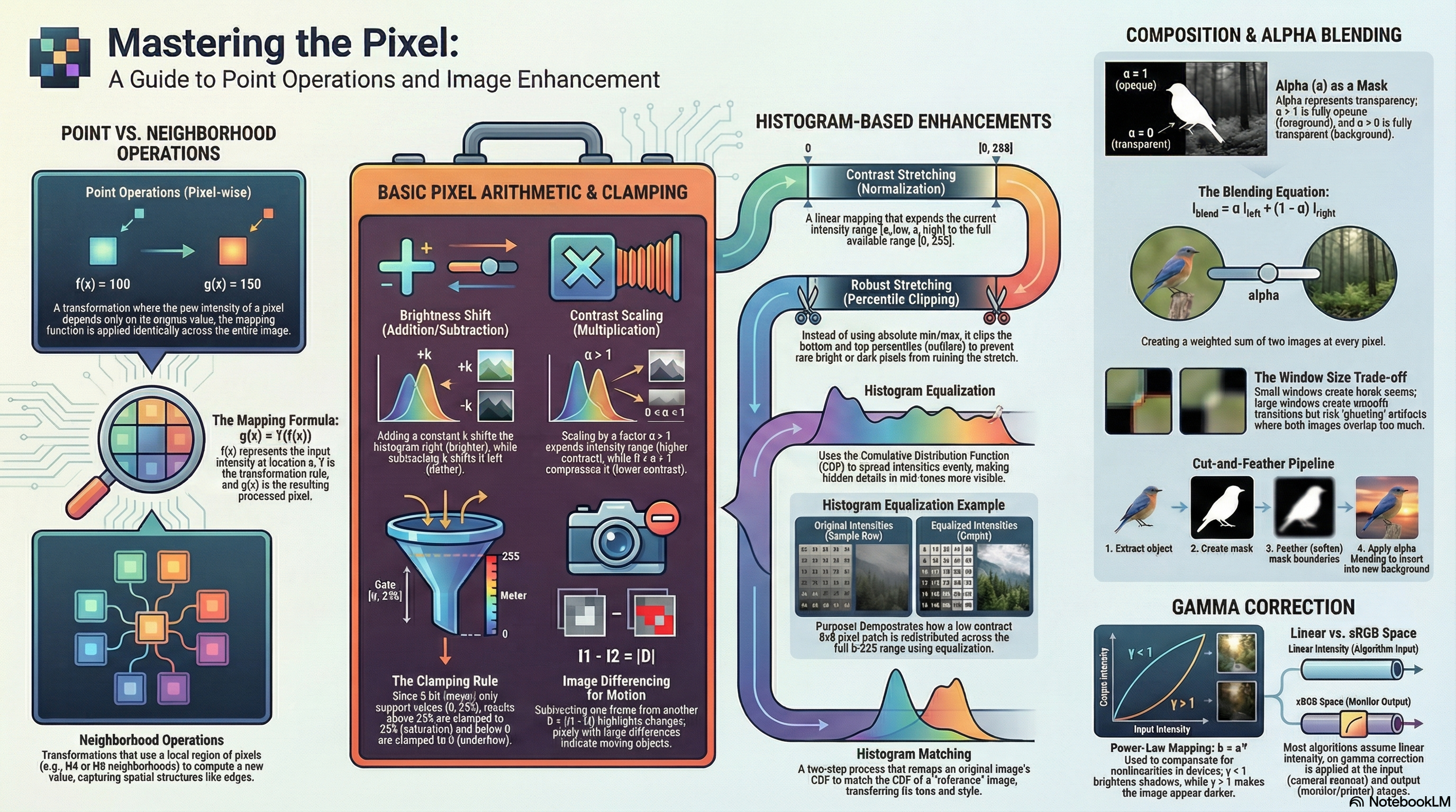
Point Operations: Change each pixel's intensity based solely on its own original value: I'(u,v) = f(I(u,v)). Spatially invariant and independent of neighbors.

Neighborhood Operations: Compute new intensities using a local spatial region around each pixel: I'(u,v) = f(I(u,v), N(p)) (e.g., filtering, resampling).

Why Define Neighborhoods Early?

Baseline Contrast: Essential to distinguish point operations from spatial filters.

Blending Control: Dictates the spatial window width for boundary feathering.

Core Foundation: Crucial for spatial filtering, edge detection, and segmentation.

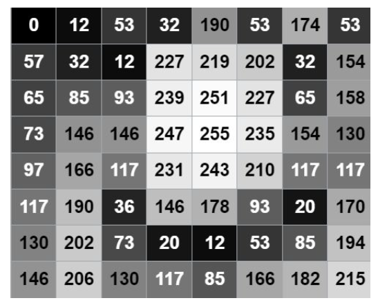
Pixel Neighborhoods & Coordinates

N₄(p) — 4-connected (Horiz & Vert)

↑

←

→

↓

{(x, y-1), (x, y+1), (x-1, y), (x+1, y)}

Nᴅ(p) — Diagonal-connected (Corners)

↖

↗

↙

↘

{(x-1, y-1), (x+1, y-1), (x-1, y+1), (x+1, y+1)}

N₈(p) — 8-connected (N₄ ∪ Nᴅ)

↖

↑

↗

←

→

↙

↓

↘

N₄(p) ∪ Nᴅ(p) (All 8 adjacent pixels)

All point operations — reference table

Operation	Formula	Effect	Histogram	Reversible?
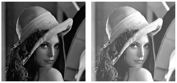
Add (k>0)	I'=clamp(I+k)	Brightens image	Shifts right	Yes (if no clamp)
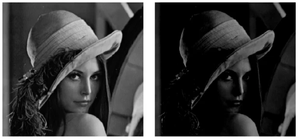
Subtract (k>0)	I'=clamp(I-k)	Darkens image	Shifts left	Yes (if no clamp)
Multiply α>1	I'=clamp(α·I)	Expands contrast	Stretch + right clip	No (clamping)
Multiply 0<α<1	I'=clamp(α·I)	Compresses, darkens	Compress leftward	Yes (if no clamp)
Invert	I'=255-I	Negative effect	Mirrors about 127	Yes
Threshold	I'=a₀ if I<a_th else a₁	Binary representation	Two spikes only	No
Quantize	I'=⌊I/Δ⌋·Δ	Reduces levels → banding	Merges bins into spikes	No

Arithmetic Range Clamping

General Clamping (Target Interval [a, b]): clamp(v, a, b) = max(a, min(b, v)) Standard 8-bit Grayscale Clamping: clamp(v) = max(0, min(255, v))

Worked Example: Pixel Addition (k = 40)

Mid-gray: I=120 → I' = 120 + 40 = 160 (brighter, details clear)

Dark: I=30 → I' = 30 + 40 = 70 (shadow details revealed)

Bright (Clamped): I=240 → 240+40=280 → clamp(280) = 255 (causes white saturation / clipping loss)

Worked Example: Pixel Subtraction (k = -70)

Mid-gray: I=120 → I' = 120 - 70 = 50 (darker, details clear)

Bright: I=200 → I' = 200 - 70 = 130 (highlights dimmed)

Dark (Clamped): I=50 → 50-70=-20 → clamp(-20) = 0 (causes black underflow / loss of shadow detail)

Clamping is not mathematically neutral: It destroys information by collapsing many different out-of-range inputs (e.g. values < 0 or > 255) into a single boundary value (0 or 255). This makes clamping operations strictly irreversible.

Image differencing — motion detection

Why |difference| is preferred

Treats both brightening and darkening equally as "change".

Clamped subtraction to 0 hides all negative differences (darkening changes are lost).

Absolute difference keeps changes in both directions fully visible.

Worked Example

No change: I₁=150, I₂=148 → |D|=2 (near zero, no motion)

Brightening change: I₁=200, I₂=120 → |D|=80 (motion detected)

Darkening change: I₁=60, I₂=140 → D=-80 → |D|=80 (motion detected; clamped subtraction would output 0)

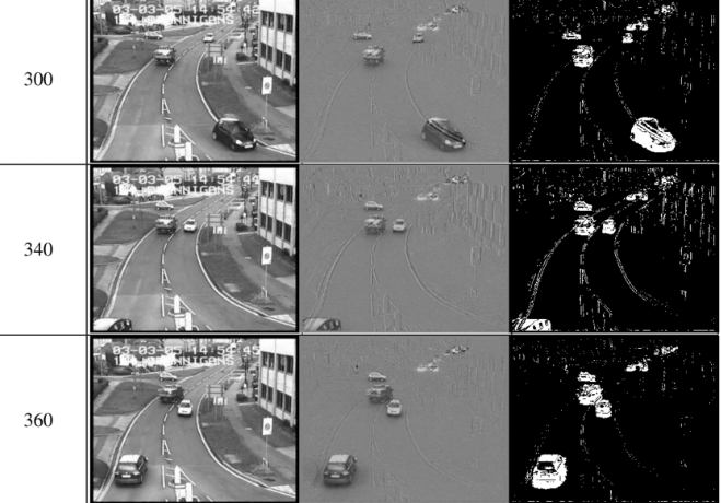
Fragmentation Concept: Motion detections via simple frame differencing can appear fragmented. This is because differencing highlights areas of intensity change (typically boundaries/edges of objects) rather than producing a solid segmentation of the moving object itself.

Quantization formula

Δ = 256 / L (L = desired number of levels) I'(u,v) = ⌊ I(u,v) / Δ ⌋ × Δ Example: L=4, Δ=64 I=100 → ⌊100/64⌋×64 = 1×64 = 64 I=150 → ⌊150/64⌋×64 = 2×64 = 128

Irreversibility of Quantization: Since multiple distinct input levels are mapped into a single coarse output bin (bin merging), the original fine details are permanently lost, introducing visual banding (contouring) artifacts in smooth gradients.

Contrast stretching

Simple Contrast Stretching (Image Normalization)

Find the actual minimum intensity $a_{low}$ and maximum intensity $a_{high}$ in the image, then linearly stretch the range to the target display interval $[0, 255]$.
Limitation: A single extreme noise pixel (outlier) can dominate $a_{low}$ or $a_{high}$, squashing the normal image details into a narrow range and keeping the image visually flat.
Key Property: Because simple contrast stretching is a linear mapping, it preserves the relative ordering of pixel intensities.

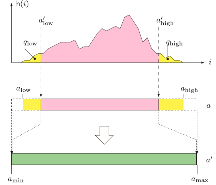
Robust Contrast Stretching (Percentile Clipping)

Instead of stretching based on absolute min/max, we choose two percentiles $q_{low}$ and $q_{high}$ (e.g., $1\%$ and $99\%$), treating values outside this range as outliers and clipping them.

a'_low = intensity at q_low percentile a'_high = intensity at q_high percentile General Piecewise Mapping to range [a_min, a_max]: a' = a_min, if a ≤ a'_low a' = ⌊ (a − a'_low) × (a_max − a_min) / (a'_high − a'_low) ⌋ + a_min, if a'_low < a < a'_high a' = a_max, if a ≥ a'_high Special Case for Standard 8-bit [0, 255] Range: a' = 0, if a ≤ a'_low a' = ⌊ (a − a'_low) × 255 / (a'_high − a'_low) ⌋, if a'_low < a < a'_high a' = 255, if a ≥ a'_high

Visual effect: The central mass of the histogram is redistributed across the full dynamic range, increasing perceived contrast. The yellow tails of the histogram outside the percentiles are intentionally saturated (clipped) to the minimum or maximum values.

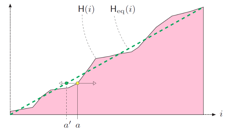
Histogram equalization

Goal & Motivation

Redistribute intensities so the histogram becomes approximately uniform (equal pixel counts per bin). Instead of simple linear endpoints, it uses the Cumulative Distribution Function (CDF) of the intensities to map pixel values.

Cumulative Histogram (CDF counts): H(a) = ∑_{i=0}^{a} h(i) (where h(i) is the pixel count of intensity i) Normalized Cumulative Distribution Function: CDF(a) = H(a) / (M · N) (where M·N is the total number of pixels) Discrete Mapping Formula (stretching with H_min offset): f_eq(a) = ⌊ (H(a) − H_min) × (K − 1) / (M·N − H_min) ⌋ Standard Normalized Mapping (8-bit): a' = ⌊ (K − 1) × CDF(a) ⌋ (where K = 256 gray levels)

Steepness contrast effects

Steep CDF regions: High pixel density (spikes in histogram). Spreads these values out, expanding contrast.

Flat CDF regions: Low pixel density. Compresses these values, reducing contrast.

Uniformity: Spreads out mid-tones, making hidden details visible.

Limitation

Noise Over-amplification: Can over-amplify noise in large homogeneous flat regions (e.g. skies).

Global Bias: Remaps globally, ignoring local spatial structure.

Adaptive Solution: Motivates local/adaptive variants (e.g., CLAHE).

Histogram matching (specification)

Tonal Style Transfer

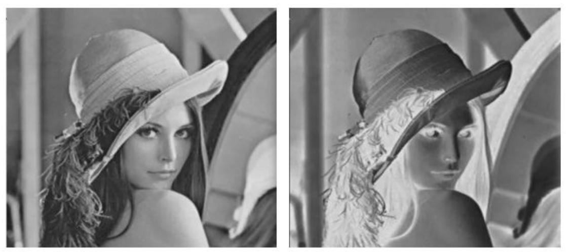
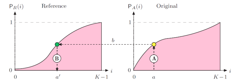
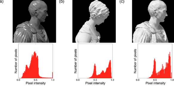
Reshape the input image's histogram to match a reference image's distribution rather than a uniform one. The image keeps the original pixel rank order, but its tonal distribution changes to adopt the reference's style.

Step 1: Map original intensity a to probability: b = P_A(a) (where P_A is the CDF of the original image) Step 2: Map probability b to reference intensity using inverse CDF: a' = P_R⁻¹(b) (where P_R is the reference image's CDF) Combined Mapping: a' = P_R⁻¹( P_A(a) )

Preservation of Rank: Histogram matching preserves the relative rank of pixel intensities. Pixels that were brighter than others in the original image remain brighter in the output image, but the absolute intensity values are shifted to match the style of the reference image.

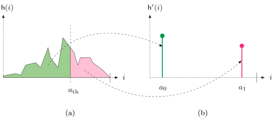
Histogram-based thresholding

I'(u,v) = a₀ if I(u,v) < a_th (typically a₀=0, black) I'(u,v) = a₁ if I(u,v) ≥ a_th (typically a₁=255, white)

Effect on histogram

Still a point operation — each pixel decided independently by comparing to a fixed threshold a_th. All values collapse into only two output levels, producing two spikes at a₀ and a₁. This is the simplest entry point to image segmentation.

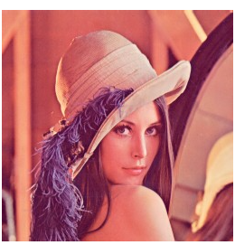
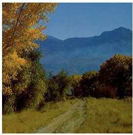
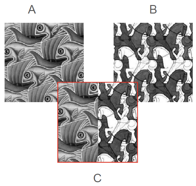
Alpha as a transparency mask

What α means

α (alpha) is a per-pixel weight, normalized to [0,1] (or stored as an extra 0–255 channel, RGBA). α=0 → no contribution; α=1 → full contribution. Conceptually, alpha IS a mask: it decides which parts of an image are emphasized vs suppressed.

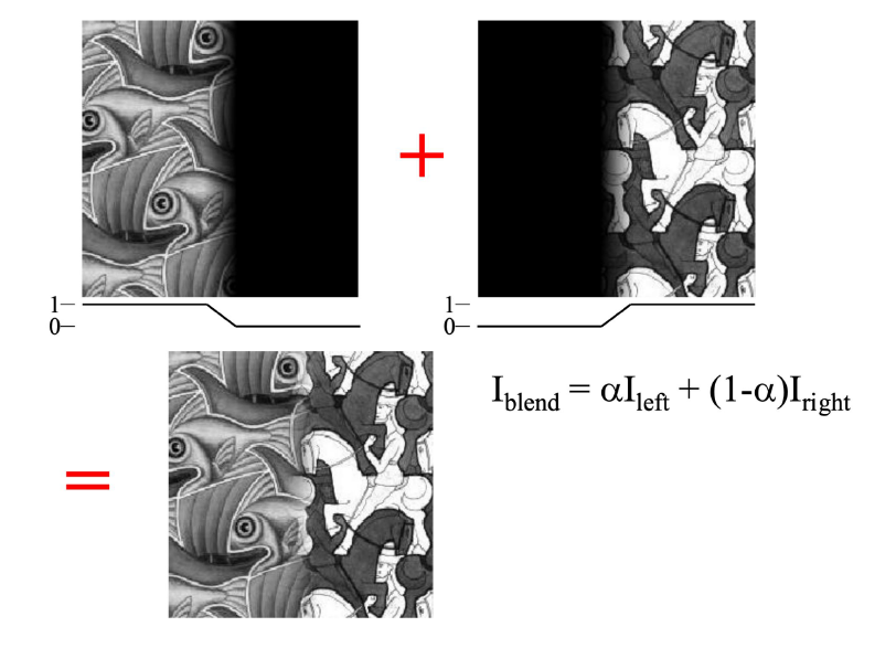
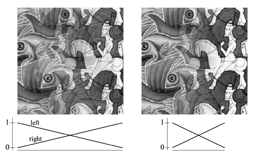
Alpha blending equation

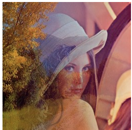
I_blend(u,v) = α·I_left(u,v) + (1−α)·I_right(u,v) Where: α = 1 → output = foreground only (I_left) α = 0 → output = background only (I_right) 0<α<1 → both contribute (double-exposure look)

Point-wise vs neighborhood

The blend equation itself is point-wise (computed independently for each pixel).

But constructing a SMOOTH alpha mask near boundaries is a neighborhood-based step (feathering/spatial windows).

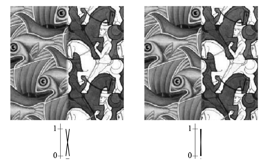
Why constant α looks "ghosty"

If α is approximately constant across the image, edges from BOTH images stay visible in the same region.

Result = transparent overlap (double-exposure), not a clean composite.

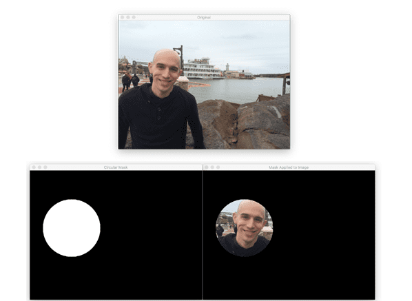
Masking — binary vs soft

Binary mask

Each pixel comes entirely from image A or entirely from image B (mask value is exactly 0 or 1). Boundary between regions appears harsh, producing a "cut-and-paste" look.

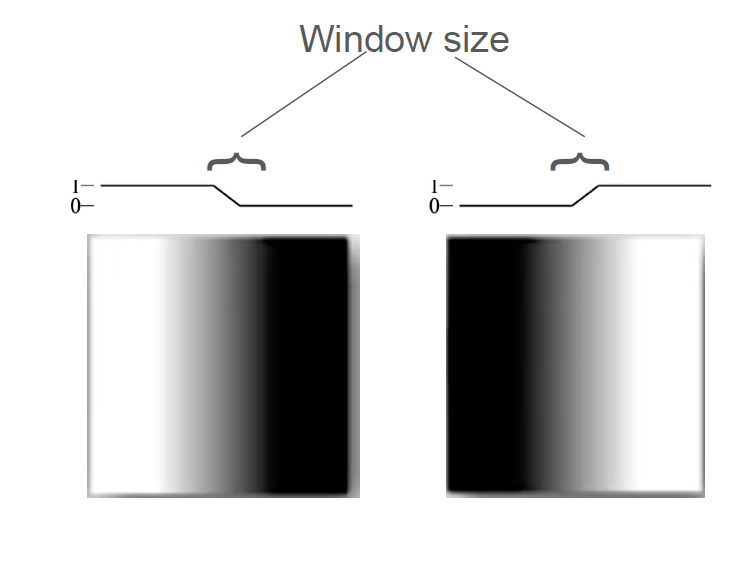
Soft mask

Mask values lie between 0 and 1. The boundary becomes a smooth transition, which is mathematically equivalent to alpha blending near the seam.

Feathering and window size trade-off

I(x,y) = w_L(x)·I_L(x,y) + w_R(x)·I_R(x,y) (per-pixel blend across spatial overlap window)

Small window

Narrow transition region.

Preserves sharp detail.

Risk: visible seam if the two images differ strongly.

Large window

Broad, smooth transition.

Improves smoothness.

Risk: ghosting (double exposure look where both images are partially visible).

Ghosting & Seams: Ghosting occurs when the transition window is too wide (or images are misaligned), so edges and textures from both sources remain partially visible simultaneously, appearing as multiple copies of objects. If the window is comparable to the full image width, the composite resembles a global blend rather than a local seam correction. A well-chosen window is "smooth enough" to hide the seam but "narrow enough" to avoid double-image artifacts.

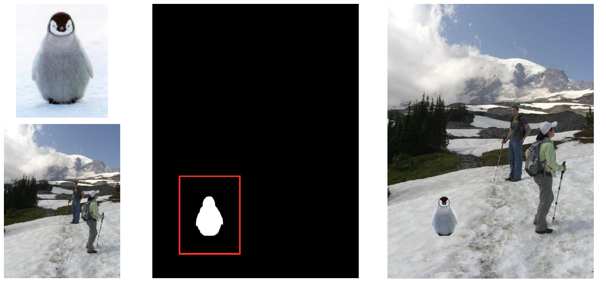
Cut-and-feather compositing pipeline

1Extract (Cut): Extract the foreground object that we want to insert into the target image, producing a foreground image F and an associated mask region.

2Feather: Modify the mask near the boundaries (feathering) so that it transitions gradually between 0 and 1. This reduces the visual discontinuity at the seam.

3Blend: Compute the output using alpha blending: I = αF + (1−α)B, where F=foreground, B=background, and α=per-pixel feathered mask value.

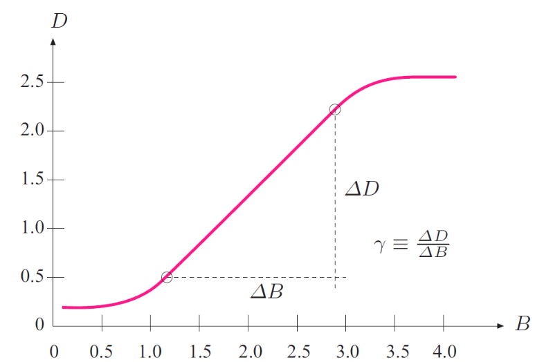
Physical Origin of Gamma

Photographic Film Response

In analog photography, film density $D$ is approximately linear with respect to log-exposure $B$ over a wide mid-range. The slope of this linear region is defined as gamma ($\gamma$).

γ ≡ ΔD / ΔB (slope of linear region of film response curve)

Historical Motivation (TV Signals)

Historically, gamma correction was applied to television broadcast signals before transmission. This was done to compensate for the non-linear transfer characteristics of cathode-ray tube (CRT) receivers. Applying the correction at the transmitter side minimized the complexity and cost of the display electronics in millions of home receivers.

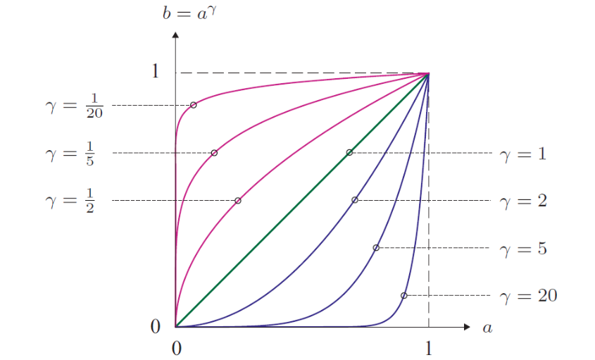
Power-law mapping

b = f_γ(a) = a^γ, a ∈ [0, 1] (normalized intensity)

γ < 1 (Expansion)

Expands dark intensities.

Shadow details become brighter and more visible.

Curve bows upward (above the identity line).

γ > 1 (Compression)

Compresses dark intensities.

Image becomes darker overall.

Highlights receive relatively more emphasis, bowing downward.

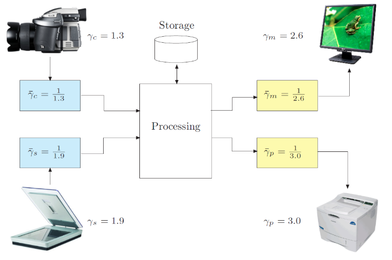
Role in the digital imaging pipeline

Linear Space Processing

Modern digital imaging pipelines process pixel values in a linear intensity space whenever possible. This is because standard image operations (such as spatial filtering, denoising, resizing, blending, and physical simulation) assume that light intensities behave linearly.

Gamma correction (or sRGB non-linear transfer functions) is applied at the boundaries of the pipeline: at raw image capture (to match sensors) and at display time (to match the human eye's perception and monitor characteristics).

Takeaway: $\gamma=1$ is the identity mapping (no change). $\gamma \ne 1$ is a single-parameter non-linear point operation that reshapes the entire tone curve, redistributing brightness without needing full cumulative histograms.

Clamp / point-operation calculator

Pick an operation, enter pixel value(s), see the clamped result.

Operation

Pixel value I120

Parameter (k / α / threshold / L)40

Alpha blending preview

α0.50

I_left220

I_right40

Gamma curve calculator

γ1.00

Input a (0–1)0.30