Lecture 3: Digital Images

What a sensor physically is

Photon buckets — the key mental model

Each pixel behaves like a photodiode (potential well) that accumulates electrons as photons strike it during exposure. Charge is proportional to light intensity × exposure time. When the well fills to its limit, saturation occurs. After exposure, the analog front-end (AFE) reads the photosites row-by-row, converting the charge into analog voltage signals, which are then converted to digital values by the analog-to-digital converter (ADC).

Photons

→

Sensor photosite
_{electrons accumulate}

→

AFE
_{analog voltage}

→

ADC
_{digital value}

→

RAW image

The complete capture pipeline

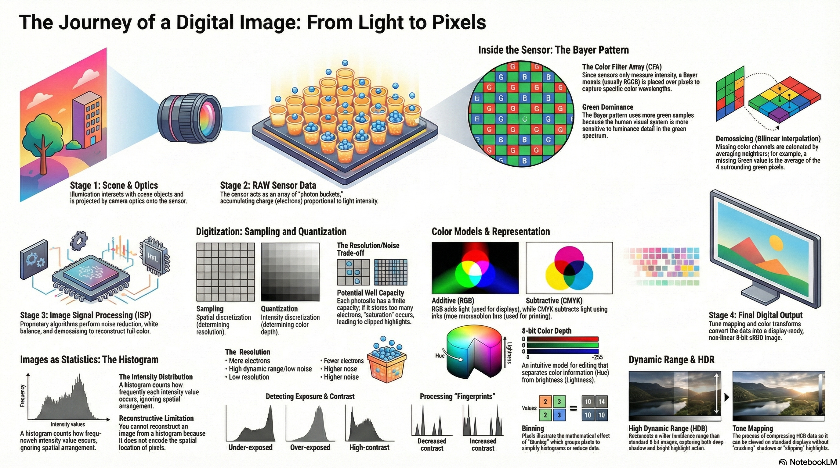
From Light Source to Digital File

Turning physical light in the scene into a digital file saved on storage involves the following sequential stages:

Light Source

→

Subject

→

Lens

→

Microlens

→

Mosaic Filter (CFA)

→

Image Sensor

→

Analog Electronics

→

ADC

→

Digital Processor

→

Buffer Memory

→

Storage (Card)

Structure of a photosite

Vertical Stack Layer Sequence (Top-to-Bottom)

Each individual pixel photosite is structured vertically as a stack of different layers:

1. Microlens_{focuses incoming rays}

→

2. Color Filter_{filters specific spectrum (R, G, or B)}

→

3. Photosite_{converts photons to charge}

→

4. Potential Well_{accumulates generated electrons}

Pixel size trade-off

Larger pixels

Bigger potential well → higher full well capacity (holds more electrons)

Higher dynamic range (more information collected before saturation)

Better low-light / SNR (larger surface area collects more photons)

Lower spatial resolution (at same physical sensor size)

Smaller pixels

Smaller potential well → lower full well capacity (saturates faster)

Higher spatial resolution (finer spatial sampling detail)

More noise sensitivity (fewer photons collected per photosite)

Reduced dynamic range (highlights clip and shadows crush quicker)

Fundamental trade-off: Resolution vs. noise performance. You cannot maximize both simultaneously.

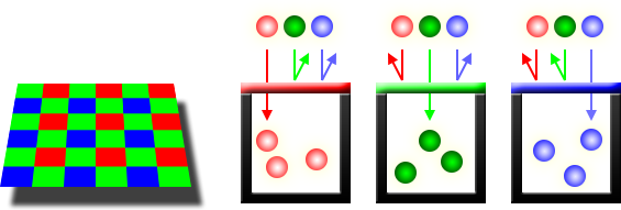
Color Filter Array (CFA) and Bayer pattern

Each photosite can only measure ONE color component (R, G, or B). A CFA mosaic places color filters above each pixel. The Bayer pattern uses 2 green, 1 red, 1 blue per 2×2 block — because human vision is most sensitive to luminance detail, which green carries.

Bayer RGGB pattern

Demosaicing (bilinear example)

At a center R pixel (R=100), average the neighbors:
G ≈ (80+84+78+82)/4 = 81
B ≈ (30+32+28+34)/4 = 31
Result: (R,G,B) = (100, 81, 31)
Not simple averaging — must preserve edges, avoid artifacts.

Why 2 greens? Luminance perception in human vision relies heavily on the green channel. More green samples → better luminance resolution → sharper-looking images.

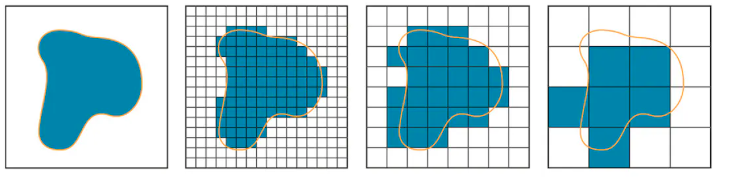
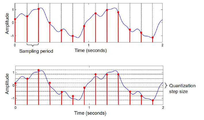
The two digitization processes

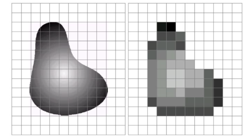
Sampling

What: Measure analog signal at discrete spatial points

Determines: Spatial resolution (pixel grid density)

Sampling Rate: Defined as the number of samples per unit spatial area.

Trade-off: Higher rate yields finer detail and less aliasing, but increases storage, bandwidth, and compute.

Artifact: Pixelation / aliasing

Quantization

What: Map continuous intensity measurements to discrete numeric levels

Determines: Intensity (color) depth

Trade-off: More levels improve approximation accuracy, but require more bits per pixel and raise storage/transmission costs.

Artifact: Quantization noise / banding

Key distinction: Sampling = WHERE you measure (spatial). Quantization = HOW PRECISELY you record the value (intensity).

Bit depth and levels

8-bit grayscale

256 levels (0–255)

8-bit RGB (24-bit)

256³ = 16.7M colors

12-bit RAW

4096 levels per channel

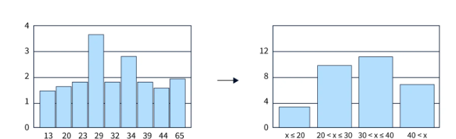
Binning

What is binning?

Groups neighboring pixels (e.g. 2×2 block) and combines their values. Reduces spatial resolution but increases SNR (more photons per "super-pixel"). Also used in histograms to group intensity ranges into coarser buckets for readability.

Input 6×6 Pixel Matrix: [ [ 2, 3, 2, 2, 3, 2 ], [ 2, 3, 5, 5, 3, 2 ], [ 2, 3, 6, 6, 2, 1 ], [ 2, 3, 6, 6, 2, 1 ], [ 3, 8, 8, 6, 4, 2 ], [ 3, 6, 5, 5, 5, 5 ] ] → Apply 2×2 Block Binning (Summing blocks) → Output 3×3 Pixel Matrix: [ [ 10, 14, 10 ], [ 10, 24, 6 ], [ 20, 24, 16 ] ]

Binning benefits

Better SNR (more signal per pixel)

Smaller data size

Binning costs

Lower spatial resolution

Hides fine tonal structure

Irreversible loss of detail

In-Camera Image Processing (ISP) pipeline

RAW to conventional RGB steps

1. RAW→ 2. Pre-processing→ 3. Noise reduction→ 4. Demosaicing→ 5. White balance→ 6. Color transform I→ 7. Color manip.→ 8. Tone mapping→ 9. Color transform II→ 10. sRGB Output

1. RAW: Mosaiced, linear, 12-bit data preserving sensor measurements.

2. Pre-processing: Basic sensor corrections (black-level offset removal, fixed-pattern noise correction, sensor non-ideality compensation).

3. Noise reduction: Suppresses photon and electronic readout noise before further processing.

4. Demosaicing: Reconstructs missing color channels at each pixel based on CFA patterns.

5. White balance: Compensates for illumination color casts so neutral objects appear neutral.

6. Color transform I: Maps sensor-dependent colors into an intermediate, device-independent space.

7. Color manipulation: Adjusts hue, saturation, and global color appearance for aesthetic preferences.

8. Tone mapping: Non-linear intensity transformation to match human perception and limited display dynamic range.

9. Color transform II: Converts intermediate coordinates to target output color space (sRGB).

10. sRGB Output: Non-linear, display-ready 8-bit RGB image.

Key exam fact: Many CV failures originate from early ISP stages (noise, demosaicing, white balance), not the vision algorithm itself.

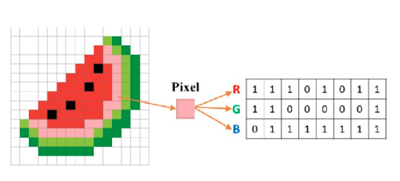
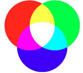
RGB — additive model

Colors formed by adding light. Each channel: 0–255 in 8-bit. Additive mixing:
Red + Blue = Magenta Green + Blue = Cyan Red + Green = Yellow R+G+B = White
Canonical: Black=(0,0,0) White=(255,255,255) Red=(255,0,0)

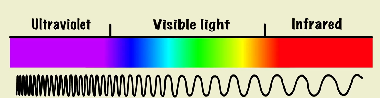
Why Red, Green, and Blue (RGB)?

Physiological Connection to Human Vision

The choice of Red, Green, and Blue as primary colors is directly rooted in human biology: the spectral sensitivities of the cone cells in our retinas. The human eye has three types of cones:

S-cones (Short-wavelength): Sensitive to Blue.
M-cones (Medium-wavelength): Sensitive to Green.
L-cones (Long-wavelength): Sensitive to Red.

Separation & Gamut: Choosing R, G, and B primary colors maximizes the physical separation between cone responses. This separation enables a large, practical color gamut, allowing monitors and projectors to reproduce a wide range of humanly perceivable colors via additive mixing.

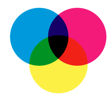
CMY / CMYK — subtractive model

Colors formed by subtracting light via inks/pigments. CMYK adds K=Black separately — more efficient than mixing C+M+Y at full intensity. Used ONLY for printing. Not suitable for digital image sensing or processing.

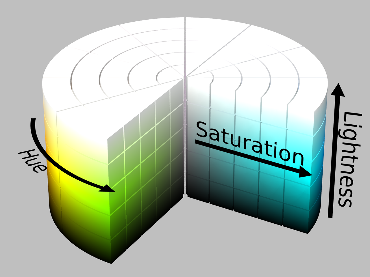
HSL / HSV — intuitive separation

Hue

Angle on color wheel (0°–360°)
0°=Red · 60°=Yellow · 120°=Green
180°=Cyan · 240°=Blue · 300°=Magenta

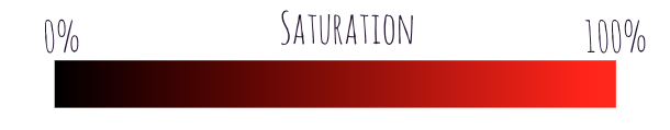
Saturation / Lightness / Value

S: 0%=gray → 100%=pure color
L (HSL): 0%=black · 50%=mid · 100%=white
V (HSV): 0%=black · 100%=brightest

RGB → HSV conversion formulas

Normalize R,G,B ∈ [0,1] first V = max(R, G, B) minVal = min(R, G, B) diff = V - minVal S = diff / V [if V ≠ 0, else S = 0] If diff == 0: H = 0° Else: If V == R: H = 60 × (G − B) / diff If V == G: H = 120 + 60 × (B − R) / diff If V == B: H = 240 + 60 × (R − G) / diff If H < 0: H = H + 360

RGB → HSL conversion formulas

V_max = max(R,G,B), V_min = min(R,G,B) diff = V_max - V_min L = (V_max + V_min) / 2 If diff == 0: S = 0 Else: If L < 0.5: S = diff / (V_max + V_min) If L ≥ 0.5: S = diff / (2 − (V_max + V_min)) H = same as HSV formula above (if diff == 0 then H = 0)

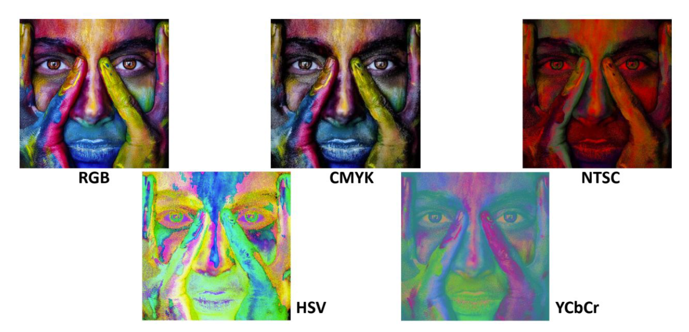
All color spaces at a glance

Space	Components	Use case	Key limitation
RGB	R, G, B	Cameras, displays, DL	Mixes brightness + color
HSV/HSL	Hue, Sat, Val/Light	Segmentation, tracking	Not perceptually uniform
YCbCr	Y, Cb, Cr	Video compression, face det.	Less intuitive visually
CMYK	C, M, Y, K	Printing only	Not for digital sensing
HSI	Hue, Sat, Intensity	Medical, satellite, agri	Limited standardization

What is pixel intensity?

Digital Representation of Measured Light

In a digital image, intensity is the discrete numeric value assigned to a pixel representing the integrated light energy measured at that photosite. It is the result of the sensor's charge readout being amplified, conditioned, and digitized by the Analog Front-End (AFE) and ADC.

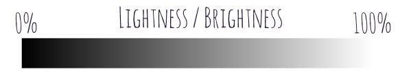
For 8-bit grayscale images, intensity is stored as an integer from 0 (completely dark/black) to 255 (completely bright/white).

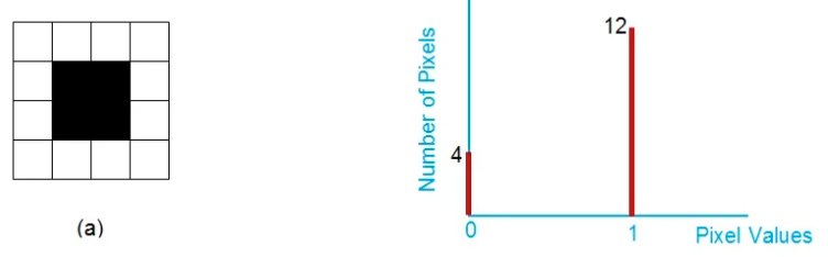
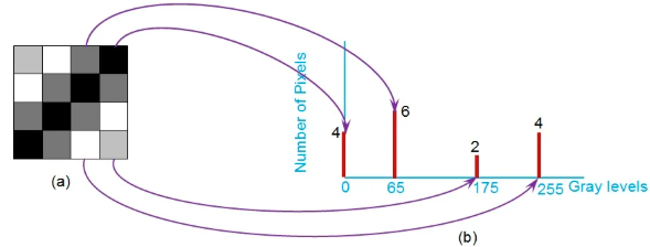
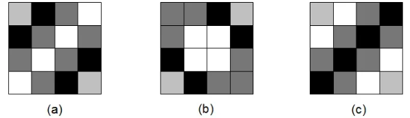
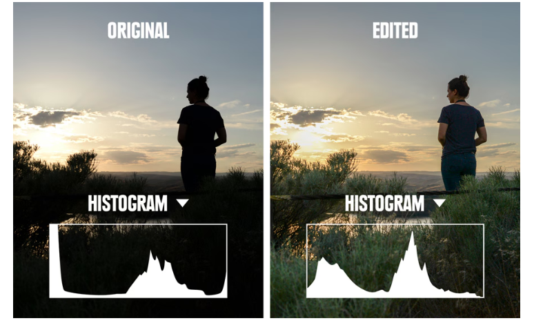
What a histogram is

A count of how many pixels have each intensity value. X-axis = intensity (0–255 for 8-bit). Y-axis = pixel count. A statistical summary — it completely discards spatial information.

Critical limitation: Two images with completely different spatial structures can have identical histograms. You CANNOT reconstruct the original image from its histogram alone. This is fundamental, not a bug.

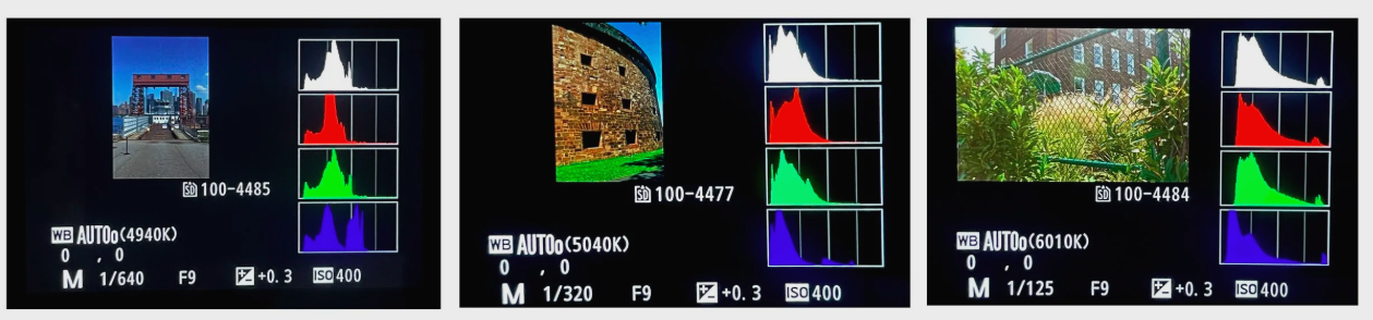
Reading histograms — what each shape means

Under-exposed

Counts concentrated at LOW values

Image looks dark / muddy

May have clipping at 0

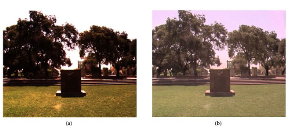
Over-exposed

Counts concentrated at HIGH values

Image looks washed out

May have clipping at 255

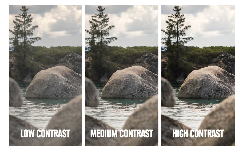
High contrast

Wide spread across full range

Objects easily distinguishable

Large min-to-max difference

Low contrast

Narrow band of values

Objects hard to distinguish

Compressed tonal range

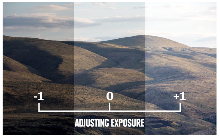
Exposure effects on histogram

↓ exposure → histogram shifts left ↑ exposure → histogram shifts right Severe clip → spike at 0 or 255

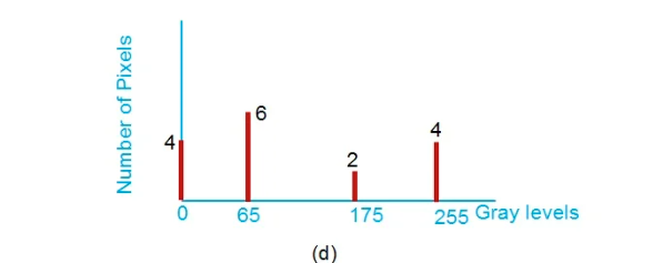
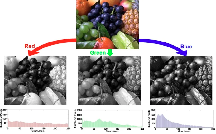
Color histograms — two approaches

Per-channel (R, G, B separately)

Shows each channel's distribution

Good for: lighting, saturation, dynamic range

Problem: Two images with different colors can have identical R/G/B histograms — the marginal distributions lose color relationships

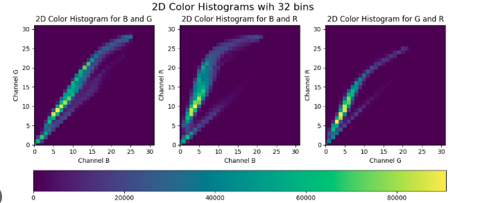
Joint / 2D histogram

Shows relationship between two channels

X=channel1, Y=channel2, brightness=count

Diagonal = strong correlation

Requires aligned, same-size images

Why per-channel isn't enough: Marginal distributions don't capture joint color relationships. A red image and a cyan image can have identical G and B histograms if the counts align. Use 2D/joint histograms to resolve this ambiguity.

Histogram artifact fingerprints

Saturation / clipping

Large spike at 0 (crushed shadows) or 255 (blown highlights). Caused by under/over-exposure or out-of-range ISP operations.

Gaps in histogram

Empty bins between occupied bins. Signature of contrast INCREASE / stretch operation — bins get spread apart.

Spikes / compression

Tall isolated spikes. Signature of contrast DECREASE — multiple values get merged into one bin. Also appears after GIF quantization (few colors → few occupied bins).

JPEG compression

Modifies intensity distribution. Creates characteristic patterns in the histogram due to DCT coefficient quantization.

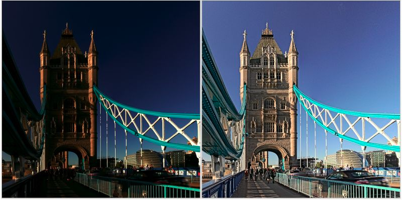
Dynamic range — core definitions

LDR (Low Dynamic Range)

Single exposure, typically 8-bit.

Cannot capture deep shadow detail and bright highlights simultaneously.

Forces a compromise: either highlights clip (sky blows to white) or shadows crush (dark areas lose detail).

HDR (High Dynamic Range)

Multiple bracketed exposures combined, or high-precision RAW formats.

Faithfully preserves details at both exposure extremes.

Requires tone mapping to compress range for standard displays.

HDR ≠ many tones. Wide dynamic range just means the range between darkest and brightest is large. You can still have few distinct tones within that range (due to quantization). Conversely, narrow dynamic range can have many tones densely packed.

HDR acquisition strategy

Bracket exposures, then merge

Capture same scene at e.g. −2EV, 0EV, +2EV. Combine: shadow detail from bright exposure, highlight detail from dark exposure. Result: HDR image → tone-map for display.

Tone mapping

Compresses wide luminance range into displayable 8-bit range. Keeps detail in both shadows and highlights visible. Strongly affects the "look" of the image. Not reversible — once tone-mapped, original HDR data is not recoverable.

Key practical rule

Capture HDR, then downsample. It's easy to reduce dynamic range from a wide capture. It's impossible to recover clipped or saturated data — interpolation cannot recreate missing information once the sensor saturated or quantization removed it.

Detecting processing artifacts via histograms

Histogram pattern	What caused it	Effect on image
Spike at 0 or 255	Clipping due to severe under-exposure or over-exposure.	Irreversible loss of shadow or highlight detail.
Gaps between bins	Contrast increase / stretch (values are pushed apart).	Posterization / visible banding.
Spikes at regular intervals	Contrast decrease / squeeze (multiple values merged).	Flat, low-contrast washed areas.
Fewer occupied bins & empty spaces	GIF compression or heavy color quantization.	Distinct posterized bands instead of smooth gradients.
Altered frequency patterns	JPEG compression (high-frequency DCT coefficient quantization).	Block artifacts and ringing along high-contrast boundaries.