Lecture 2: Image Formation

The core equation

I(x,y) = R(x,y) · L(x,y)

I(x,y)

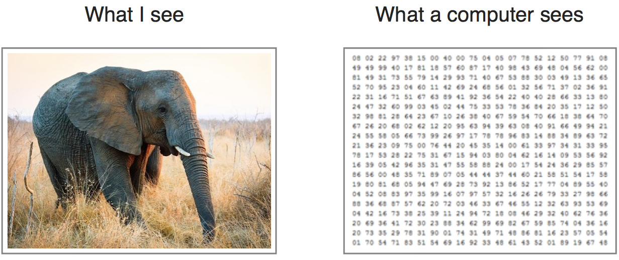
Measured intensity — what the camera actually records

R(x,y) — Reflectance

Intrinsic surface property. Ideally invariant to lighting. Encodes color + material.

L(x,y) — Illumination

How light arrives at the surface. Varies over time & scene.

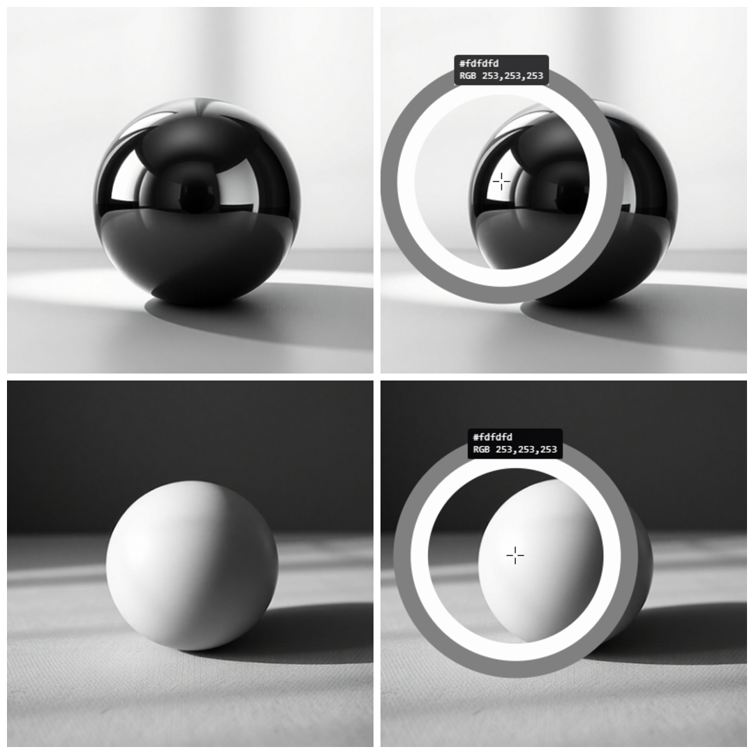
Key ambiguity: The same pixel value can come from a bright surface in shadow OR a dark surface under strong light. A computer can't tell them apart without extra info.

Example: Intrinsic Ambiguity Calculation

Linear Mapping to 8-bit Grayscale

Assume a linear mapping model where:

pixel_value = (I / 1000) · 255, where I = R · L

Let's compare two different scene points that produce the exact same pixel intensity:

Pixel A (Bright surface in shadow):
Reflectance R_A = 0.80 (80% reflecting), Illumination L_A = 250 units.
Intensity: I_A = 0.80 · 250 = 200.
Pixel Value = (200 / 1000) · 255 = 51.0
Pixel B (Dark surface under strong light):
Reflectance R_B = 0.20 (20% reflecting), Illumination L_B = 1000 units.
Intensity: I_B = 0.20 · 1000 = 200.
Pixel Value = (200 / 1000) · 255 = 51.0

Both Pixel A and Pixel B map to the same digital value (51.0), meaning the camera records them identically, losing the distinct physical attributes of color and lighting.

Two pillars of image formation

Geometry

Controls: Structure & shape

Q: Where does a 3D point land?

Determined by: Camera pose, focal length, FOV, projection model

Photometry

Controls: Appearance (brightness/color)

Q: How bright/what color is that point?

Determined by: Illumination, reflectance, sensor response

What algorithms try to do with I=R·L

Suppress L(x,y) — illumination

Normalize away shadows, shading, time-varying light → illumination normalization, gradient-based features, ratio representations

Preserve R(x,y) — reflectance

Capture material/texture/color for reliable recognition, matching, segmentation → reflectance-based features

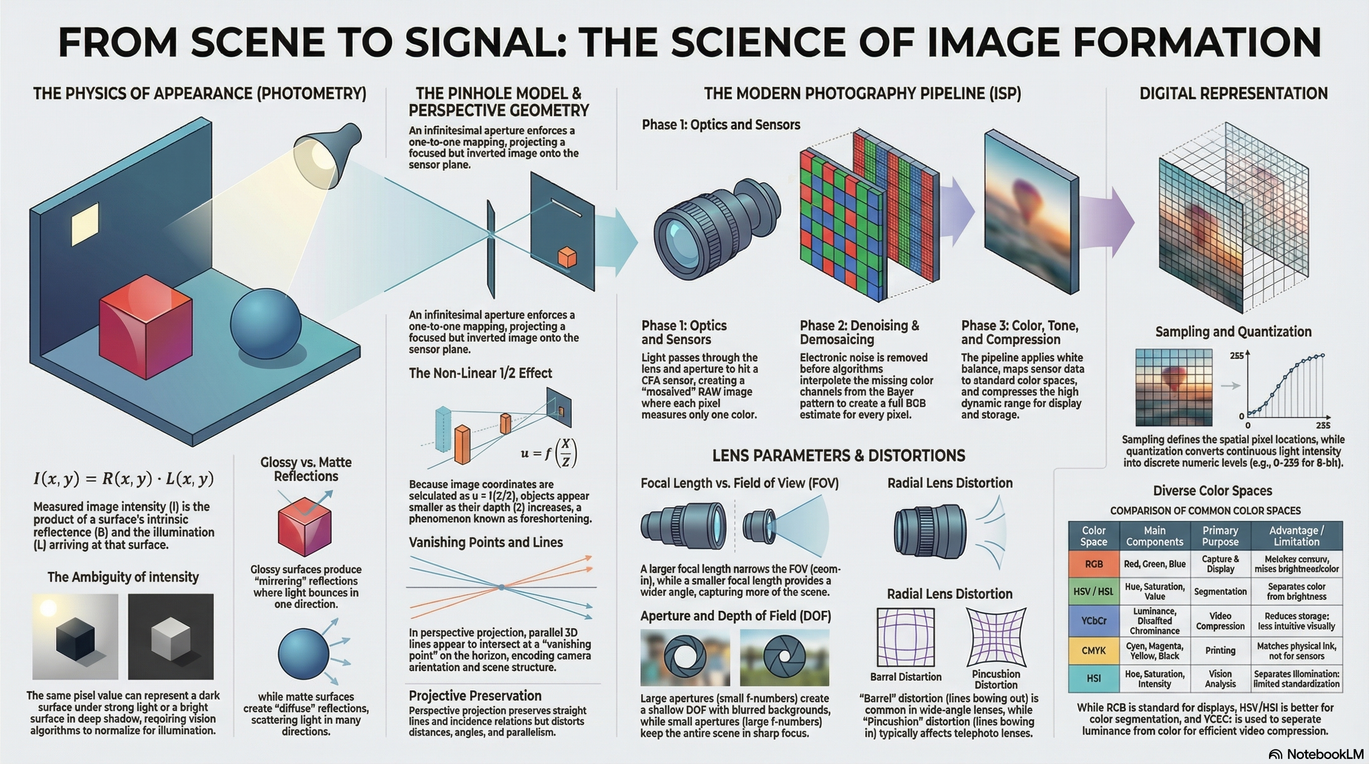
From Scene to Digital Image — Concept Map

Scene Interaction & Photometry

Real World Scene (geometry + materials) → Illumination (light sources, shadows) → Light-Surface Interaction (reflectance/material) → Photometry / Appearance (brightness, color, shading) modeled as I(x,y) = R(x,y) · L(x,y).

Imaging Geometry

Real World Scene (geometry + materials) → Imaging Geometry (pinhole, projection, field of view (FOV), depth of field (DOF)). Determines where 3D points project on the 2D plane.

Camera System Integration

Imaging Geometry + Photometry / Appearance → Camera System (optics + sensor + ISP). Combines physical projection rays with measured light intensities.

Optical & Digital Processing

Camera System → Optical Imperfections (lens distortion) + Digital Representation (sampling, quantization, coordinate grids) + Color Representation (RGB and other color spaces).

✓

Final Output

Optical Imperfections + Digital Representation + Color Representation → Final Digital Image (grid of pixels as digital numbers).

Mental model: We do not "see objects" — we measure light.

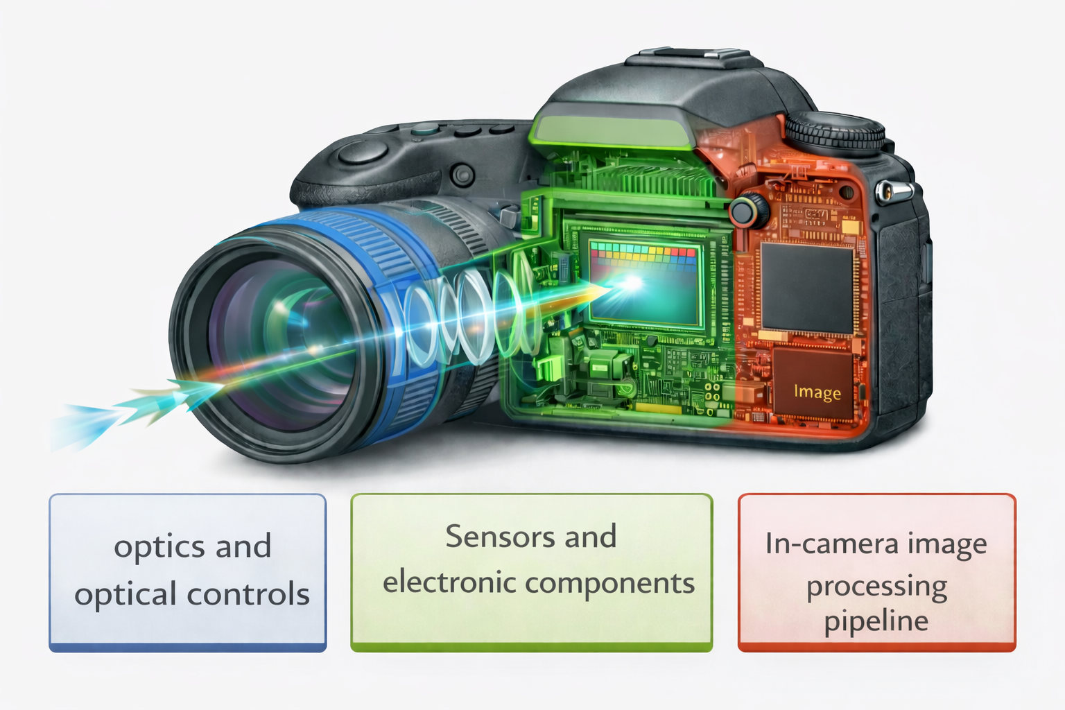
The Photography Pipeline: 3 Distinct Phases

Phase 1: Optics

Optics & Optical Controls

Light enters through the physical camera lens and is restricted by the aperture.
Components: Lens Elements, Aperture, Shutter, Focus Mechanism.

Phase 2: Sensors

Sensors & Electronic Components

Photons strike the Color Filter Array (CFA) sensor and generate analog voltages, which are conditioned by the Analog Front-End and digitized.
Intermediate Output: RAW Image (Mosaiced, Linear, 12-bit).

Phase 3: Digital ISP

In-Camera Image Processing Pipeline

The RAW image goes through digital processing steps:

1. Denoise 2. Demosaic 3. White Balance 4. Color Transform 5. Tone Reproduction 6. Compression

Final Output: RGB Image (Full Color, Non-linear/Gamma-encoded, 8-bit).

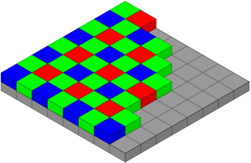
Understanding Sensor Mosaicing & Bayer Pattern

What is a Mosaiced RAW Image?

A digital camera sensor does not measure full RGB color at each pixel. Instead, it is covered by a Color Filter Array (CFA). Each individual pixel measures only one color component: Red (R), Green (G), or Blue (B).

The spatial arrangement of these filters forms a mosaic pattern, commonly called the Bayer Pattern (a repeating 2×2 grid containing 2 Green filters, 1 Red filter, and 1 Blue filter per block). More green is used because the human eye is most sensitive to green luminance/detail.

G R
B G

Because each pixel contains only a single intensity value, the raw sensor output looks black-and-white. The demosaicing step mathematically interpolates neighboring values to reconstruct the missing color channels and create a full-color RGB image.

RAW vs final RGB — key differences

RAW image (after sensor)

Color: Mosaiced (1 channel/pixel)

Linearity: Linear w.r.t. scene radiance

Bit depth: 12-bit

Viewable? No — requires ISP processing

Final RGB image

Color: Full RGB at every pixel

Linearity: Non-linear (gamma encoded)

Bit depth: 8-bit per channel

Viewable? Yes — standard display format

Each ISP step — what it does & why

1. Denoising

Removes photon noise + electronic noise from RAW. Done FIRST so noise isn't spread into all channels by demosaicing. Over-denoising destroys texture.

2. CFA Demosaicing

Each pixel only has R, G, or B (Bayer pattern: RGGB — 2 green, 1 red, 1 blue per 2×2 block). Demosaicing estimates the 2 missing channels per pixel from neighbors → full RGB.

3. White Balance

Different light sources (sun, incandescent, fluorescent) cast different color temperatures → color cast. WB adjusts per-channel gains so neutral objects appear neutral.

4. Color Transform

Sensor RGB ≠ display RGB. Mathematical matrix maps from sensor color space to a standard display color space for consistency across devices.

5. Tone Reproduction

Real scenes have much wider dynamic range than displays. Tone mapping compresses range while preserving contrast. Defines the image's "look".

6. Compression

Encodes final image (JPEG/PNG) for storage. Trades file size vs visual quality. Lossy compression introduces artifacts.

Critical exam point: Many CV failures originate in early ISP stages (noise, white balance, demosaicing) — NOT in the vision algorithm itself.

Why can't we just view RAW directly?

Only 1 color/pixel (CFA) Linear — looks washed out 12-bit — displays are 8-bit

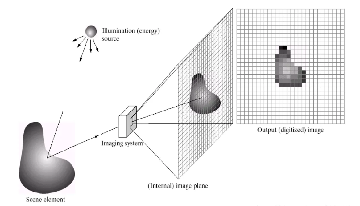
Sensors & Optical Constraints

Sensors: What They Measure

An image sensor does not measure an ideal mathematical point in the scene. Each pixel records the integrated light energy arriving at that pixel.

Integration occurs over:

• Spatial area: The pixel footprint on the image plane.

• Time interval: Exposure time (can cause motion blur).

• Spectral range: Defined by the color filter placed above the pixel.

Thus, a pixel represents an average measurement, not an exact sample.

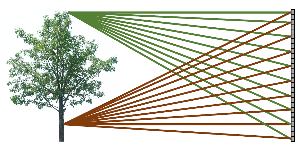
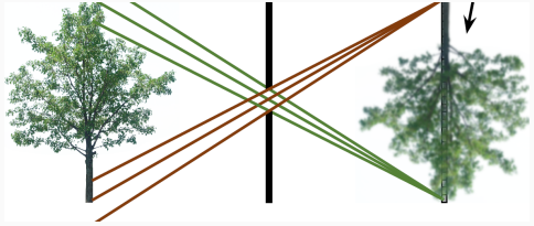
"All Points Contribute" Problem

In the absence of optical constraints (no lens or pinhole), light rays from every scene point scatter and reach every sensor pixel.

Consequences of spatial mixing:

• Each pixel contains information from multiple scene locations.

• Fine spatial details become completely indistinguishable.

• The resulting output is a completely blurred, featureless gradient.

The role of optics (lenses/pinholes) is to enforce a one-to-one mapping.

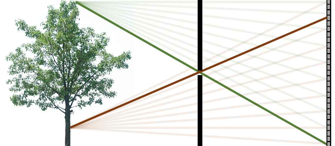
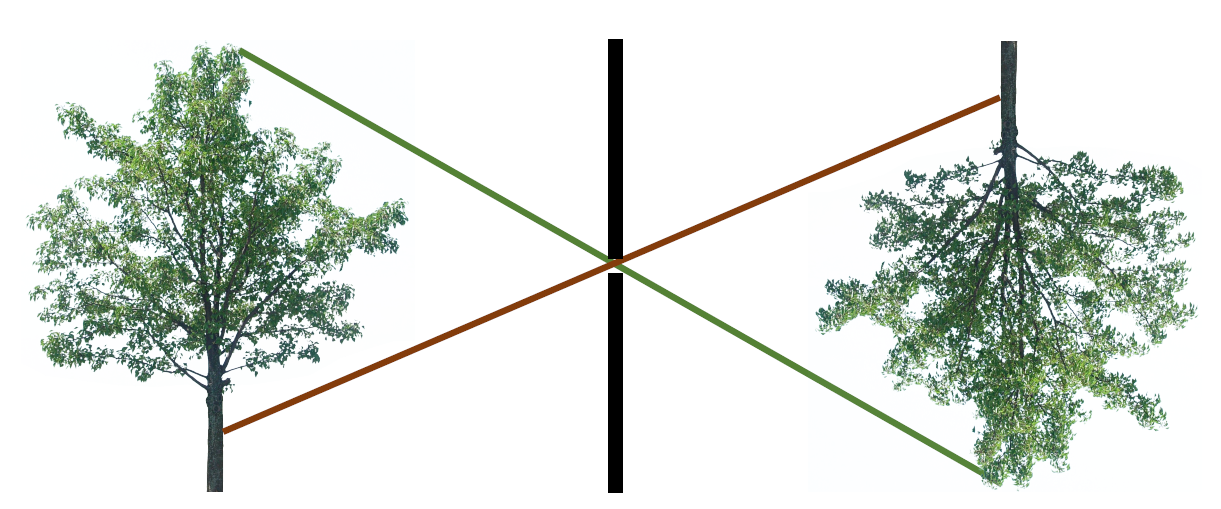
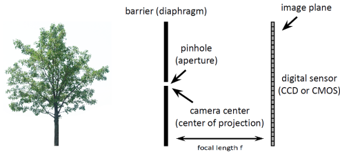
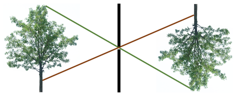
Pinhole camera model

Core principle

An infinitesimal aperture enforces a single ray path per scene point → one-to-one mapping from 3D scene to 2D image. Result: inverted image.

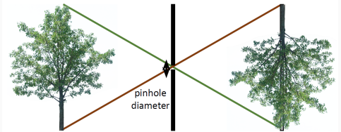
Larger pinhole

More light → brighter image

Multiple rays per point → blur

Smaller pinhole

Less light → dimmer image

Sharper until diffraction dominates

Optimal size exists — there's a sweet spot before diffraction takes over.

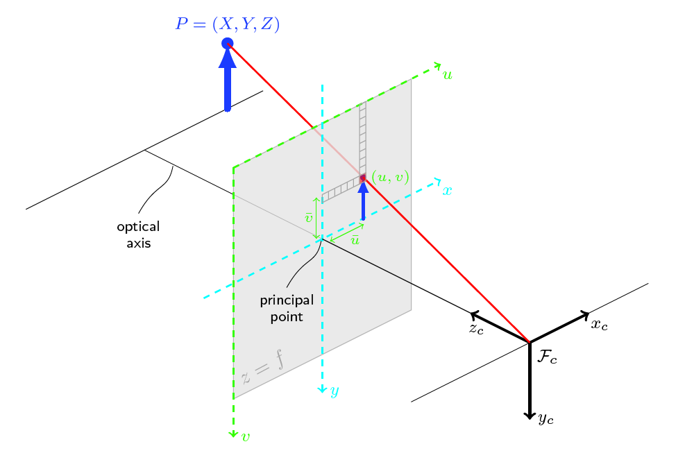
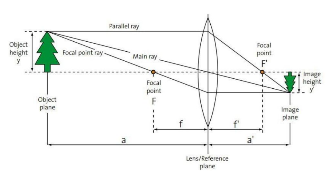
Perspective projection equations

u = f · (X / Z) v = f · (Y / Z)

(u, v)

Image point on the 2D plane

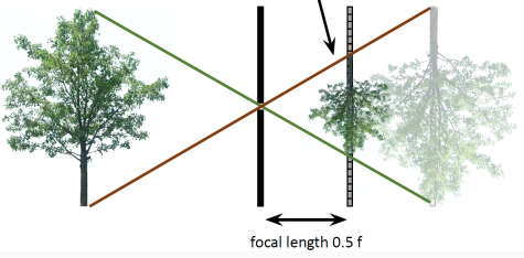
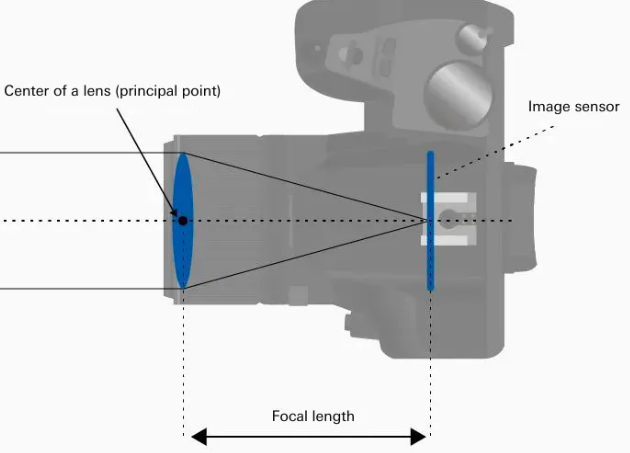
Focal length — distance from center to image plane

(X, Y, Z)

3D scene point in camera coords. Z = depth.

Consequences of the 1/Z Term

The perspective projection is non-linear due to the division by depth Z. Any two points on the same projection ray (X, Y, Z) and (λX, λY, λZ) project to the same image location (u, v), meaning depth information is lost.

Foreshortening: Objects appear smaller as depth Z increases (larger Z moves coordinates closer to the principal point).
View-dependent appearance: The same object projects to different shapes depending on camera viewpoint.
"Visual Illusions": Many visual illusions are natural geometric consequences of perspective projection rather than errors in human perception.

Magnification

m = y' / y = f / Z

Magnification decreases as depth Z increases. Derived from similar triangles. Larger f → more magnification at same distance.

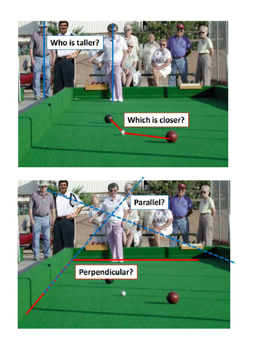
What projection PRESERVES vs LOSES

Preserved

Straight lines → still straight

Incidence relations (points on lines)

NOT preserved

Distances

Angles

Parallelism (lines can converge)

Implication: Metric measurements (real distances, angles) require camera calibration and explicit geometric modeling.

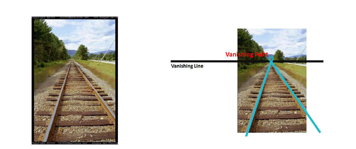
Vanishing points

Why they exist

3D parallel lines DO NOT intersect in Euclidean space. Under perspective projection they converge to a vanishing point in the image — a point at infinity in projective geometry. Railroad tracks are the classic example.

What they encode

Camera orientation (rotation), dominant scene directions. Used for: camera calibration, horizon estimation, scene understanding (roads, corridors, architecture).

Focal length trade-off

Larger f (telephoto)

Narrower FOV

More magnification (zoom-in)

Smaller scene portion captured

Smaller f (wide-angle)

Wider FOV

Less magnification

Larger scene portion visible

Important: Changing f affects magnification, NOT scene depth.

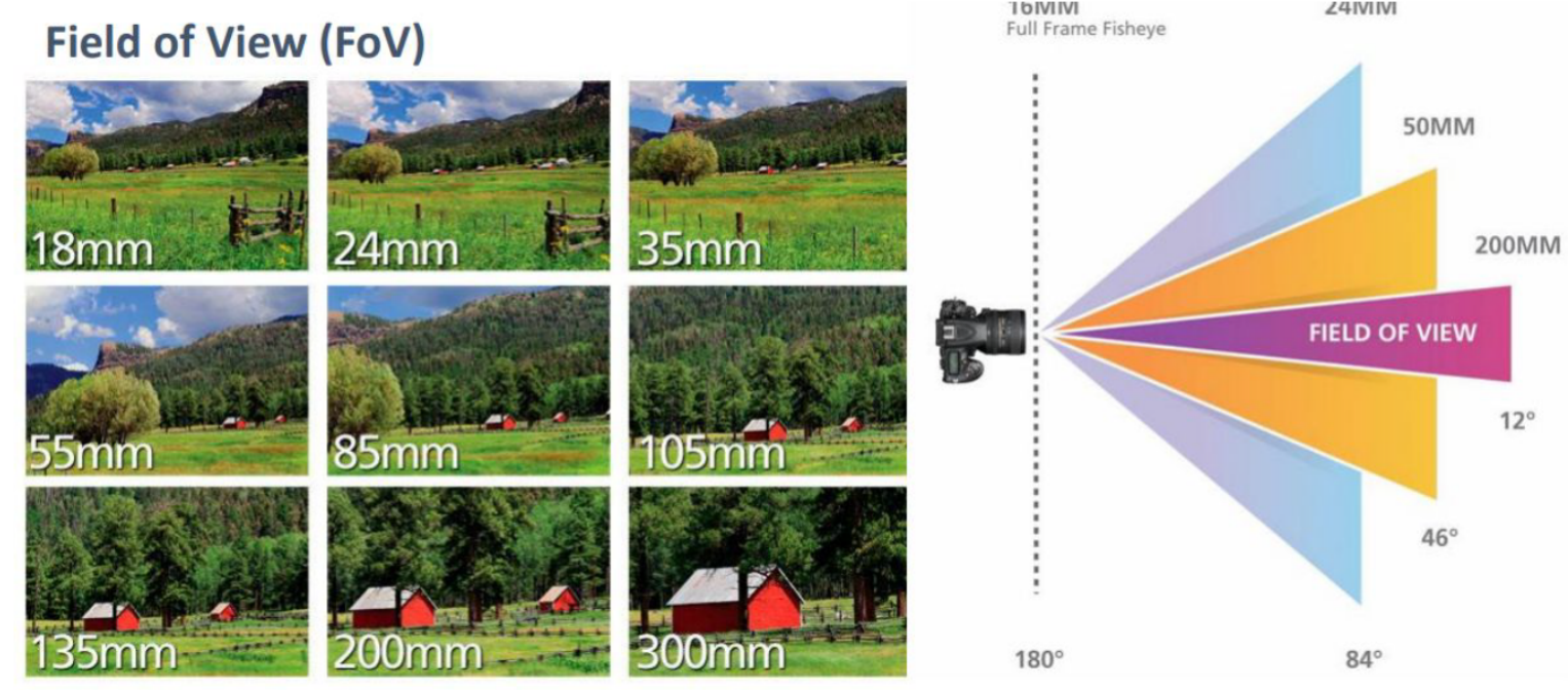
Field of View (FOV)

FOV = 2 · tan⁻¹(w / (2f))

w = sensor dimension, f = focal length. FOV depends on BOTH sensor size and focal length.

Focal Length: Increasing focal length f reduces FOV and produces a zoomed-in view.
Sensor Size: Increasing sensor size w (with fixed f) increases FOV and captures a larger portion of the scene.
Measurement: Defined in the camera coordinate system and measured with respect to the optical axis. It can be horizontal, vertical, or diagonal.
Conceptual Note: FOV describes how much of the world is visible, not how large objects appear. Object size in the image depends on both focal length and distance. It does not depend on scene depth.

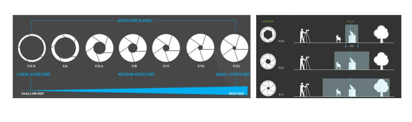
Depth of Field (DOF)

Definition

Range of scene distances that appear acceptably sharp. A consequence of finite aperture size. Points OUTSIDE DOF project to blurred circles (circle of confusion), not single points.

Large aperture (small f-number, e.g. f/2.8)

More light → brighter

Shallow DOF → strong background blur (bokeh)

Portrait / subject isolation

Small aperture (large f-number, e.g. f/16)

Less light → darker

Deep DOF → everything sharp

Landscape / architecture

DOF is optical, not projection geometry. It's about blur from aperture, not about where things project.

Why use lenses instead of pinholes?

More light collection Focus control Controllable FOV and magnification

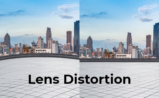
A lens approximates pinhole projection with much better light efficiency. But lenses introduce distortion.

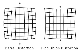
Lens distortion types

Barrel distortion

Magnification decreases from center

Straight lines bow OUTWARD

Wide-angle / action cameras

Pincushion distortion

Magnification increases from center

Straight lines bow INWARD

Telephoto / zoom lenses

r_d = r · (1 + k₁·r² + k₂·r⁴ + k₃·r⁶ + ...)

r = distance from image center. k₁, k₂, k₃ = radial distortion coefficients. Distortion is systematic → correctable through calibration. Points farther from center → larger displacement.

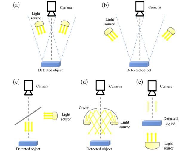
Illumination types and effects

Directional

Strong shadows, high contrast. Like direct sunlight.

Coaxial

Light along camera axis → no shadows, uniform. Used for flat reflective surfaces.

Diffuse

Soft transitions, reduced shadows. Like overcast sky or softbox.

Backlighting

Light behind subject → silhouettes, reduced front detail.

Key: Changes in illumination can dominate pixel values even when objects and camera don't move at all.

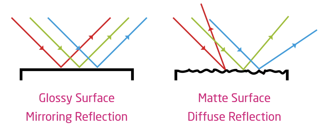
Surface reflection & material properties

Diffuse (matte)

Light scattered in all directions.

Appearance same from any angle.

Shows texture well.

Specular (glossy)

Light concentrated in highlights.

View-dependent appearance.

Can hide texture, create glare.

Transparency & Reflections: Transparent and highly reflective materials mix background colors with reflections, making their appearance depend strongly on the environment.
Color & Spectral Reflectance: Surface color depends on spectral reflectance, which determines which specific wavelengths of light are absorbed versus reflected.
Texture & Micro-geometry: Physical texture is determined by micro-geometry, which creates fine-scale shading and microscopic specular highlights.

Image as a mathematical function

Continuous: I : Ω ⊂ ℝ² → ℝᵏ Digital: I : ℤ² → ℝᵏ

k = 1

Grayscale image (single intensity value per pixel)

k = 3

Color image (RGB channels)

k = N

Multispectral / hyperspectral (multiple bands)

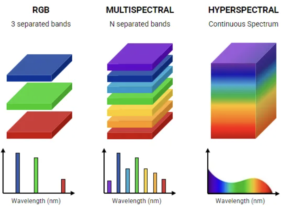
Types of Spectral Images

RGB Images

Number of Bands: k = 3

Spectrum: Three discrete channels (Red, Green, Blue).

Usage: Acquisition and display systems matching human sight.

Multispectral Images

Number of Bands: k = N (typically 3 to 10)

Spectrum: Multiple separated, discrete bands.

Usage: Standard remote sensing, satellite imaging.

Hyperspectral Images

Number of Bands: k = hundreds of narrow bands.

Spectrum: A continuous, contiguous spectral range across electromagnetic wavelengths.

Usage: Chemical analysis, precise agricultural monitoring, mineral mapping.

Sampling & quantization

Sampling

Selects discrete spatial locations

Each location = one pixel

More samples = finer spatial detail

Quantization

Converts continuous intensity to discrete levels

8-bit = 256 levels (0–255)

More bits = finer intensity resolution

Coordinate conventions

Image coordinates

Row, column indexing → (y, x)

Origin: top-left corner

Used in pixel access / arrays

Cartesian coordinates

Position as (x, y)

Used in geometric / projection math

Must specify convention to avoid bugs

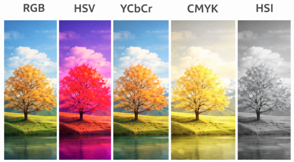
Color spaces — full comparison

RGB (Red, Green, Blue)

Acquisition & Display

Purpose & Design: Directly matches camera sensors and monitor displays. Mixes brightness and color information.

Limitations: Highly sensitive to illumination changes, making pure RGB comparison difficult under shadows or varying brightness.

Applications: Image capture, standard displays, object detection, image classification, face recognition, deep learning pipelines.

HSV / HSL (Hue, Saturation, Value / Lightness)

Segmentation & Tracking

Purpose & Design: Separates color info (Hue) from brightness (Value/Lightness) and purity (Saturation) for intuitive color-based analysis.

Limitations: Not perceptually uniform (a mathematical distance between colors doesn't map to human color perception).

Applications: Color-based segmentation, tracking object markers, traffic sign detection, skin segmentation.

YCbCr (Luminance + Chrominance Blue / Red)

Video Compression

Purpose & Design: Separates brightness (Luminance Y) from color (Chrominance Cb, Cr). Exploits human eye limits by subsampling color data.

Advantages: Significantly reduces storage/bandwidth needs. Skin tone clusters very compactly in Cb-Cr space.

Applications: Video compression (MPEG, H.264), JPEG images, broadcasting, face detection, surveillance systems.

CMY / CMYK (Cyan, Magenta, Yellow, Black)

Printing Only

Purpose & Design: Subtractive color mixing used for physical inks (reflecting light instead of emitting it).

Limitations: Completely unsuited for image sensing (cameras) or digital computer vision processing algorithms.

Applications: Industrial printing, packaging inspection, color consistency verification in production.

HSI (Hue, Saturation, Intensity)

Vision Analysis

Purpose & Design: Similar to HSV but optimized for mathematical vision analysis, separating intensity from pure color properties.

Limitations: Has limited hardware standardization, requiring color space conversions in software.

Applications: Satellite image analysis, agricultural monitoring, medical imaging, industrial surface inspection.

Why switch color spaces? RGB mixes brightness and color together — that makes many tasks harder. Alternative spaces isolate the property you care about → simpler algorithms, better robustness to lighting.

I = R × L pixel simulator

Demonstrates how two completely different surfaces can produce identical pixel values. Adjust R and L for each pixel.

Pixel A

R_A (reflectance)0.80

L_A (illumination)250

Pixel B

R_B (reflectance)0.20

L_B (illumination)1000

Perspective projection calculator

Given a 3D point P=(X,Y,Z) and focal length f, compute image coordinates (u,v).

X100

Y50