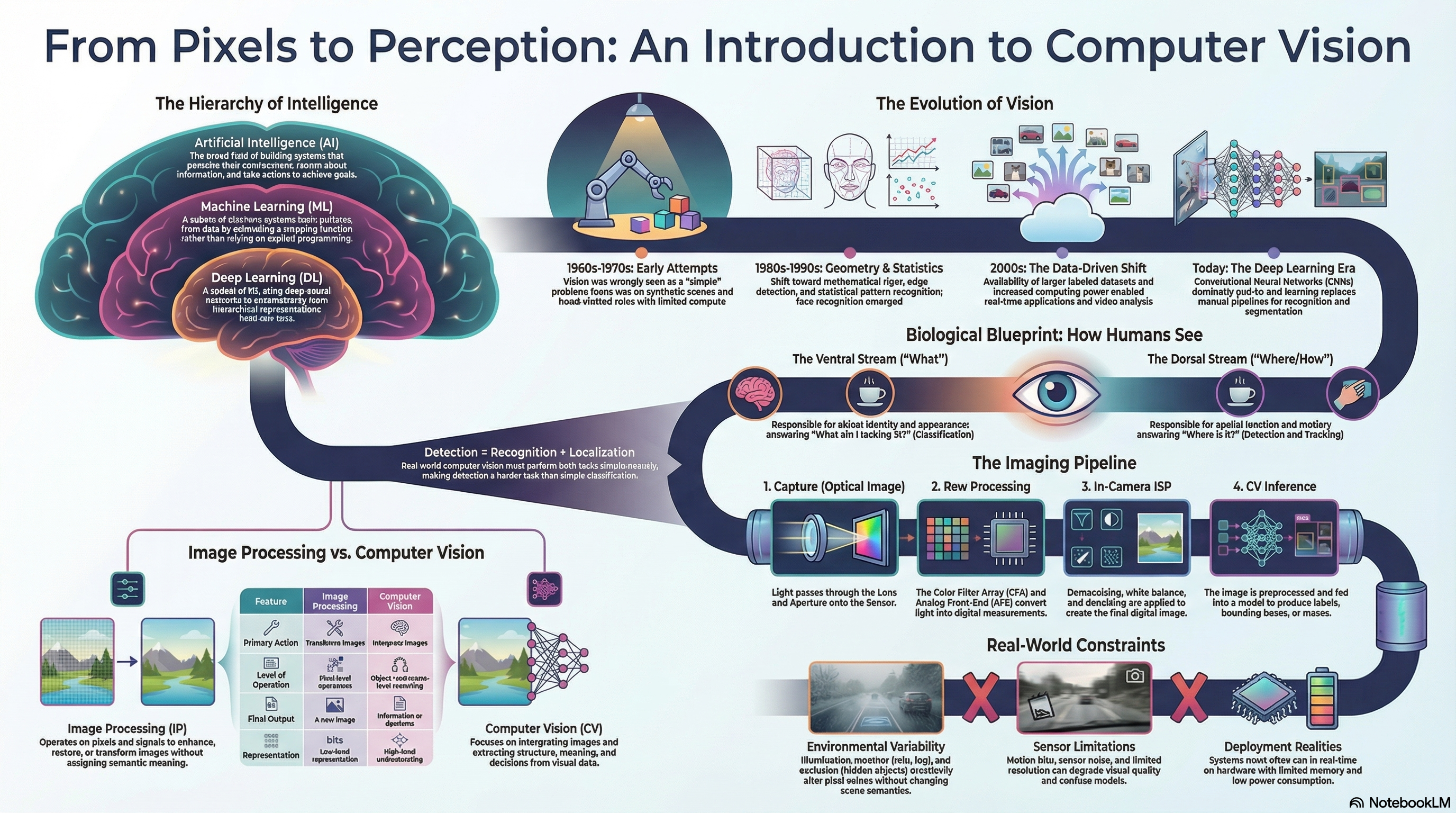
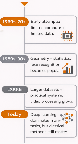
Evolution of computer vision
1960s–70s: Early attempts
Vision seen as a "simple" problem (wrong). Limited compute & memory. Synthetic scenes, hand-crafted rules and heuristics.
No dataNo compute
1980s–90s: Geometry & statistics
Mathematical rigor. Edge & corner detection, feature extraction. Statistical pattern recognition. Face recognition emerges.
SobelCannyHarris
2000s: Data-driven & practical
Larger labeled datasets. More compute. Video analysis and real-time applications grow.
SIFTSURFReal-time
Today: Deep learning era
CNNs dominate. End-to-end learning. Significant gains in recognition, detection, segmentation. Classical methods still matter for efficiency & geometry.
CNNsTransformersE2E
Progress needs 3 things simultaneously
Sufficient data
Enough compute
Sound math models
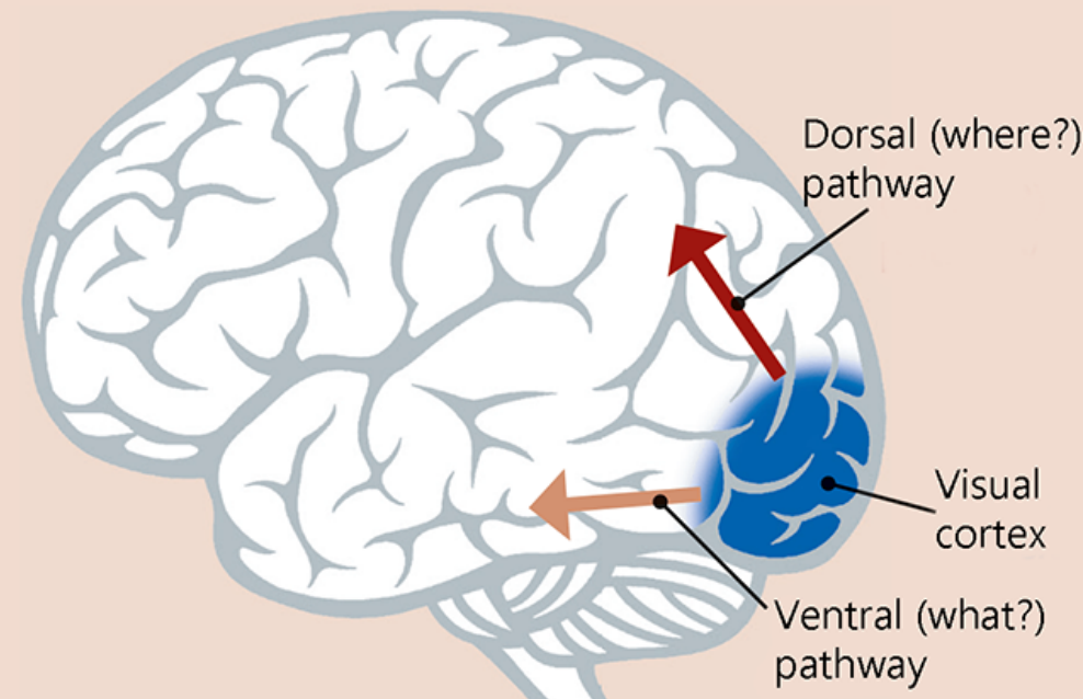
The two visual streams (biology → CV)
Ventral Stream
"What" pathway
Task: Object identity & appearance
CV equiv.: Classification / Recognition
Q it answers: What am I looking at?
Dorsal Stream
"Where / How" pathway
Task: Spatial location & motion
CV equiv.: Detection / Tracking
Q it answers: Where is it?
Key insight
Detection = Recognition (what) + Localization (where). Detection is the harder task because it requires both.
Image processing vs computer vision
Image Processing
Does: Transforms images
Level: Pixel-level operations
Output: An image
Meaning: No semantic meaning
Examples: Denoise, blur, resize
Computer Vision
Does: Interprets images
Level: Object/scene reasoning
Output: Information / decisions
Meaning: High-level understanding
Examples: Detect cars, classify faces
A captured image is NOT ground truth
Every step introduces bias/artifacts: opticssensor noiseexposurecolor processingdenoisingcompression
Real-world constraints (exam favourite)
Environment
Illumination changes, occlusion, clutter — same scene looks totally different.
Sensors & Data
Motion blur, noise, dataset bias — models trained on curated data fail in deployment.
Deployment
Real-time constraints, limited memory, low power. High benchmark accuracy ≠ robustness in the wild.
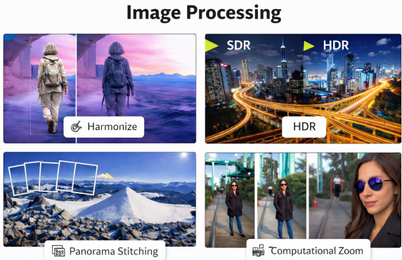
Image processing subcategories
Image Enhancement
Noise reduction, contrast adjustment, sharpening. Improves visual appearance.
Image Restoration
Denoising, deblurring, correcting sensor-level artifacts. Reverses degradation.
Geometric Transforms
Scaling, rotation, alignment, warping. Manipulates spatial coordinates.
Representation Change
Color space conversions, filtering, and frequency-domain analysis.
Computer vision core questions
What is present?
Object and scene recognition (Image Classification).
Where is it?
Spatial localization (Object Detection or Segmentation).
What is the geometry?
Depth, scale, pose, and 3D scene structure.
How does it change?
Motion estimation, object tracking, and optical flow over time.
Computer vision applications
Everyday Systems
Auto Driving: Lane/pedestrian detection, collision avoidance (Tesla, Waymo, Mobileye)
Face ID: Identity verification & authentication (Apple Face ID, Android Face Unlock)
Augmented Reality: Face filters, environment tracking (Snapchat, Instagram, TikTok)
Professional Systems
Healthcare: Tumor detection, X-ray & MRI analysis (Google Health, Aidoc)
Security: Person tracking, anomaly detection, crowd surveillance
Interaction: Gesture recognition, body tracking (Microsoft Kinect, Meta Quest)
Complete end-to-end vision pipeline
Raw Image / Video
→
Preprocessing
denoise, resize, normalize
→
Feature Extraction
corners, edges, descriptors
→
ML / DL Model
inference
→
Output
labels / boxes / masks
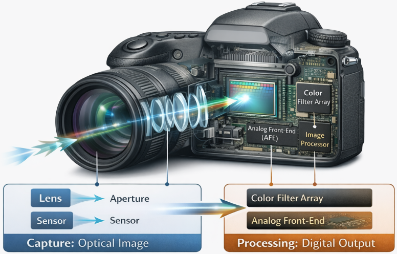
Camera imaging pipeline
Optics
lens, aperture
→
Sensor + AFE
+ CFA
→
ISP
demosaic, WB, denoise
→
Post-capture
enhance, compress
CFA = Color Filter Array | AFE = Analog Front-End | WB = White Balance | ISP = Image Signal Processor
Image processing core categories
Quantification
Sampling rate, resolution, intensity quantization, aliasing
Transformation
Geometric (scale, rotate, warp), intensity (gamma, histogram eq.)
Filtering
Linear & non-linear filters, denoising, edge enhancement, frequency domain
Analysis
Pixel stats, region properties, low-level descriptors
Classic feature extraction
Corner detection
High local intensity variation → Harris, Shi-Tomasi
Edge detection
Strong intensity gradients at boundaries → Sobel, Canny
Feature matching
Local descriptors for correspondence across images → SIFT, SURF, ORB