Lecture 12: Modern Vision Models and Applications

From Classification to Richer Vision Outputs

Recall: CNN Classifiers

A standard CNN classifier receives an image and produces a prediction about the main class represented. The output is usually a vector of class scores/probabilities, and the class with the highest score is selected as the predicted label. While image classification answers: What is the main content of this image?, it does not tell us where objects are located.

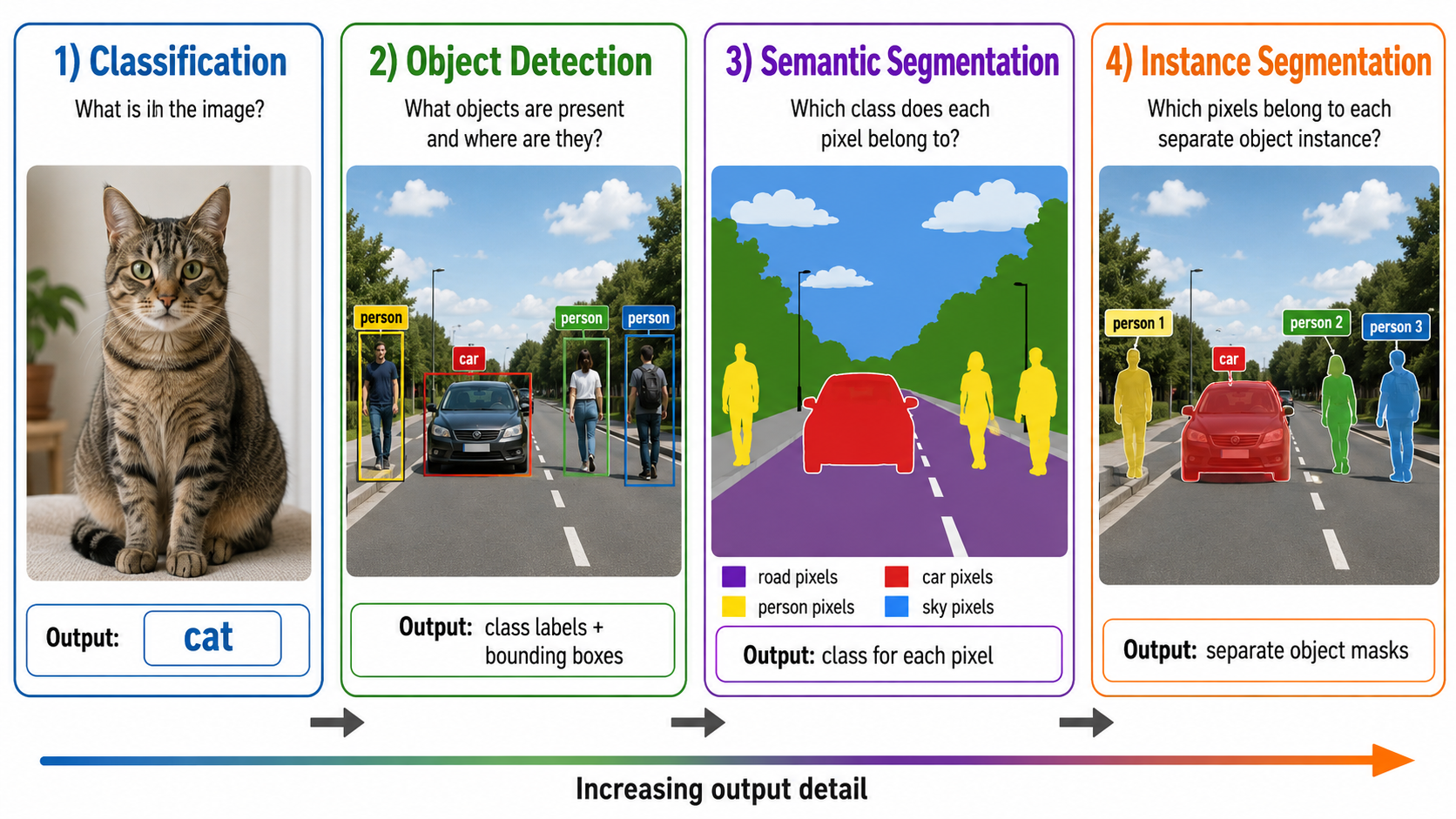
Many real-world vision applications need richer, pixel-specific, or temporal outputs. As we move from classification to tracking, the level of output detail and complexity increases.

Five Core Vision Output Types

1. Classification

What is the main content of the image?

Output: one class distribution or label for the whole image.

Does not localize objects.

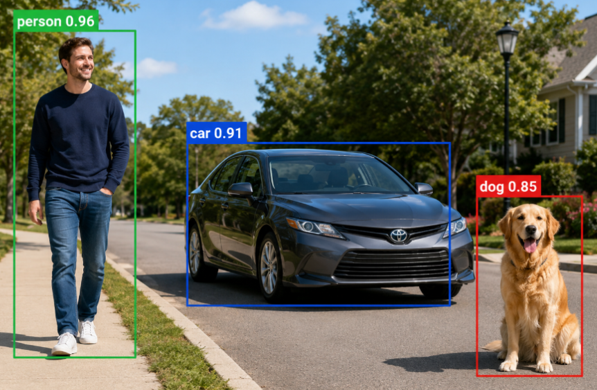
2. Object Detection

What objects exist and where are they?

Outputs: Class labels + Bounding Boxes (coordinates).

Applications: Autonomous driving, retail shelf monitoring.

3. Image Segmentation

Which class does each individual pixel belong to?

Outputs: Pixel-level class maps (semantic) or distinct boundaries (instance).

Applications: Medical diagnostics, satellite mapping.

4. Pose Estimation

What is the structural layout of key joints?

Outputs: Bounding coordinates + Joint Keypoints (shoulders, elbows).

Applications: Sports analysis, gesture control.

5. Object Tracking

Which object in this frame is the same as from previous frames?

Outputs: Dynamic bounding boxes with persistent Track IDs.

Applications: People counting, security monitoring.

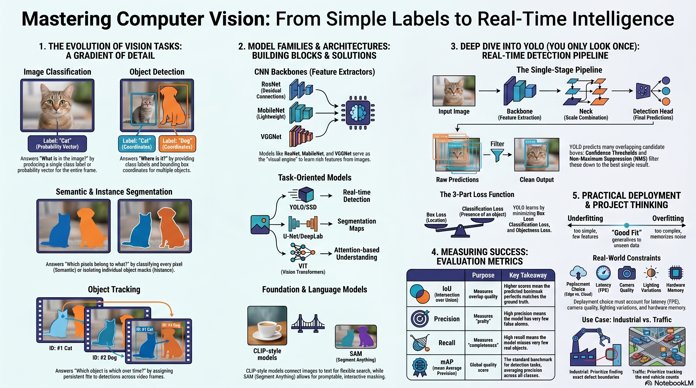
The Complexity Continuum

Moving from left to right increases output detail and complexity:
Classification ➔ Object Detection ➔ Semantic Segmentation ➔ Instance Segmentation ➔ Tracking & Video intelligence

Practical Rule: A richer output requires significantly more annotation effort, more careful metric evaluation, and more complex deployment constraints.

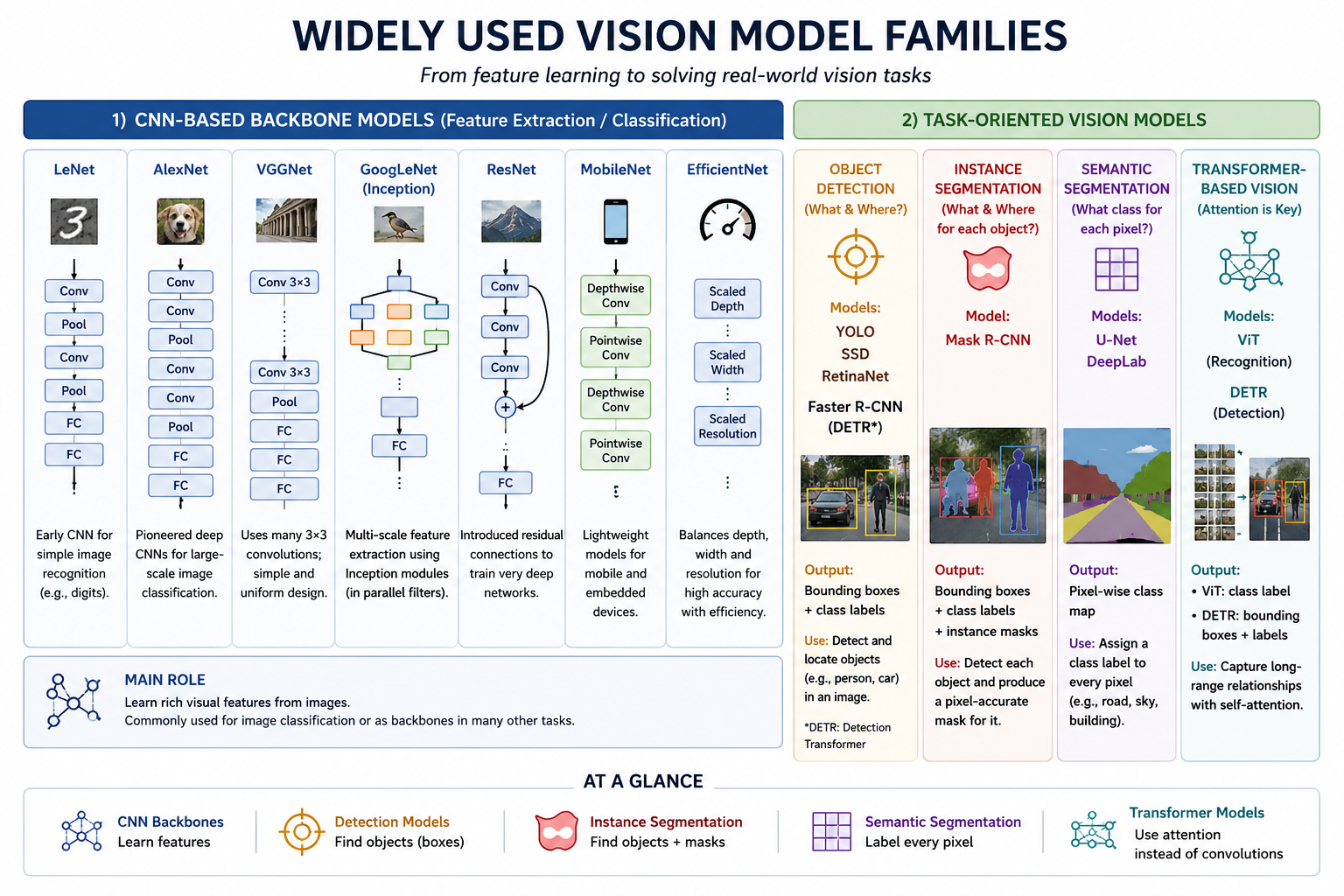
1. CNN Backbone Models (Feature Extraction)

These models are designed to learn rich visual features from images. They are commonly used for standard image classification, or act as the "backbone" inside larger task-oriented vision architectures (like YOLO or Mask R-CNN).

Early & Deep

LeNet: Early CNN for simple digit recognition (MNIST).

AlexNet: Pioneered deep CNNs on ImageNet.

VGGNet: Uniform design with stacks of $3 \times 3$ filters.

Advanced Features

GoogLeNet: Multi-scale feature extraction via Inception modules.

ResNet: Residual skip connections to train ultra-deep networks.

Efficiency Oriented

MobileNet: Lightweight depthwise separable convolutions for edge devices.

EfficientNet: Systematically balances depth, width, and resolution.

2. Task-Oriented Model Families

Model Family	Main Output	Typical Use Case / Characteristics
YOLO, SSD, RetinaNet	Bounding boxes & class labels	Single-stage, real-time object detection in video frames.
Faster R-CNN, Mask R-CNN	Region proposals, boxes, masks	Two-stage, highly accurate detection and instance segmentation.
U-Net, DeepLab	Pixel-level class maps	Semantic segmentation (medical images, satellite maps).
ViT (Vision Transformer), DETR	Attention-based labels/boxes	Uses transformer attention; original DETR still uses a CNN backbone before its transformer encoder-decoder.
SAM, SAM 2	Promptable pixel masks	Zero-shot interactive segmentation (point/box prompt input).
CLIP-style models	Image-text similarity score	Zero-shot open-vocabulary recognition & flexible search.

Two-Stage vs. Single-Stage Detectors

Two-Stage Detectors

Step 1: Propose candidate object regions (Region Proposal Network).

Step 2: Classify each proposed region and refine its box boundaries.

• Examples: R-CNN, Fast R-CNN, Faster R-CNN, Mask R-CNN.

• Typical trade-off: Proposal processing usually increases latency, although accuracy depends on the architecture, training, and evaluation setting.

Single-Stage Detectors

Predict object classes and bounding boxes directly in a single forward pass, without a separate proposal step.

• Examples: YOLO, SSD, RetinaNet.

• Typical trade-off: Efficient end-to-end inference suited to real-time systems; small/crowded-object performance depends on feature resolution and model design rather than stage count alone.

YOLO: You Only Look Once

YOLO is a family of single-stage object detection models designed to predict bounding boxes and class-related confidence scores in one forward pass. Early YOLO versions described a fixed grid of cells; modern versions generally predict at many locations over multiple feature-map scales and may use anchor-based or anchor-free heads. Exact output parameterization and post-processing are version-dependent.

Main Architectural Components

Backbone: Extracts visual features from the input image. Early layers capture primitive structures (edges, textures); deep layers capture semantic structures (object parts).

Neck: Combines features from different scales (resolutions) using feature pyramids. This is critical for detecting both small and large objects.

Detection Head: Produces box parameters and class/confidence scores at multiple prediction locations. Some YOLO variants include an explicit objectness branch; others use different confidence formulations.

Bounding-Box Representations

A box can be stored as corners $(x_1,y_1,x_2,y_2)$ or as center and size $(c_x,c_y,w,h)$: \[ x_1=c_x-\frac{w}{2},\quad y_1=c_y-\frac{h}{2},\quad x_2=c_x+\frac{w}{2},\quad y_2=c_y+\frac{h}{2}. \] Coordinates may be absolute pixels or normalized by image width and height; training and decoding must use the same convention.

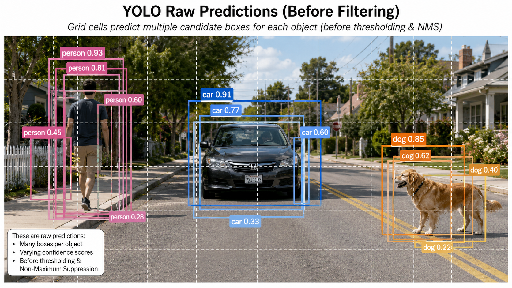
Raw Predictions & Filtering

The Need for Post-Processing

YOLO evaluates multiple locations simultaneously, producing multiple overlapping candidate boxes around the same object, plus many weak background detections. Post-processing filters this raw output:

• Confidence Thresholding: Discards any candidate whose final detection score falls below a selected threshold. How this score combines class confidence and objectness is version-dependent.
• Non-Maximum Suppression (NMS): Groups overlapping boxes belonging to the same class. It keeps the box with the highest confidence and suppresses (discards) other overlapping boxes whose Intersection over Union (IoU) exceeds a set overlap threshold.

Non-Maximum Suppression Algorithm

For boxes $A$ and $B$: \[ \operatorname{IoU}(A,B)=\frac{|A\cap B|}{|A\cup B|} =\frac{|A\cap B|}{|A|+|B|-|A\cap B|}. \]

1. Remove boxes below the confidence threshold. 2. For each class (in class-aware NMS), select the highest-scoring remaining box. 3. Keep it and suppress remaining boxes whose IoU with it exceeds tau_NMS. 4. Repeat until no candidates remain. Lower tau_NMS suppresses more aggressively. NMS is common in YOLO-style pipelines, but end-to-end set predictors such as original DETR are designed not to require NMS.

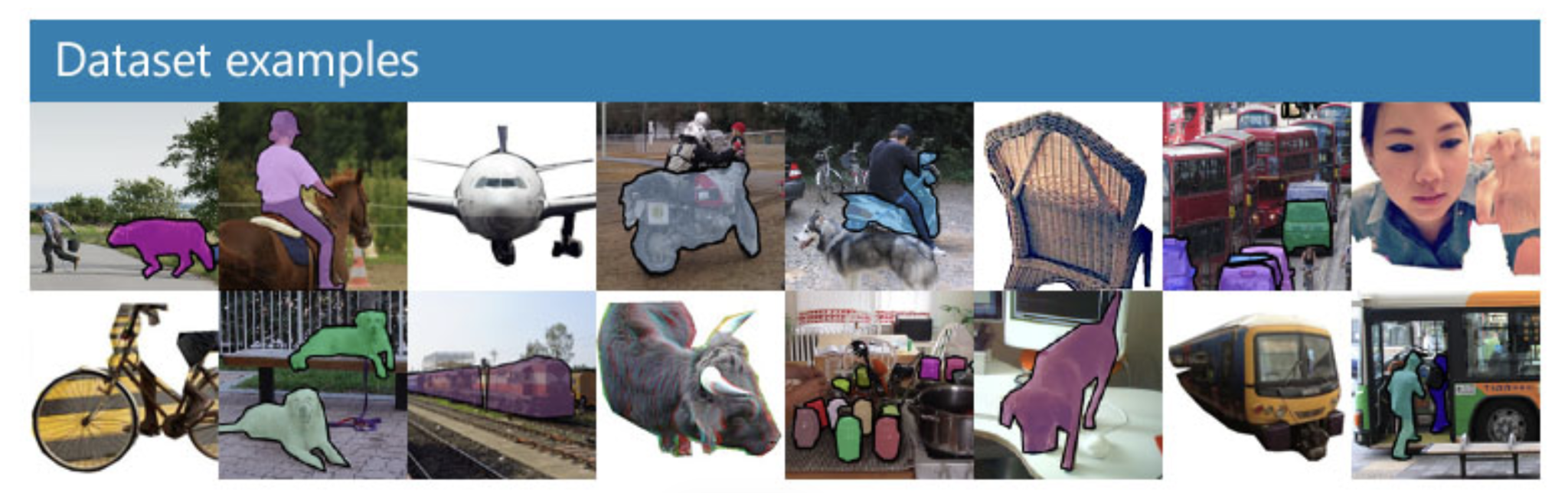
Pretraining on the COCO Dataset

COCO (Common Objects in Context) is a large-scale dataset used for benchmarking vision tasks.
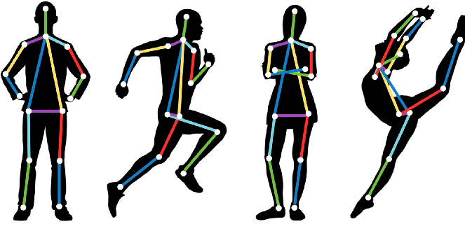
✔ Key stats: 330K images ($>200K$ labeled), 1.5 million object instances, 80 object categories (people, animals, vehicles, household items), 91 stuff categories, and keypoints for 250K people.

Pretraining a YOLO model on COCO teaches it strong general visual representations. For custom applications, engineers typically take a COCO-pretrained model and fine-tune it on their custom labeled dataset.

Object Detection Loss Function

A detector commonly minimizes a weighted multi-task objective. The exact losses and whether a separate objectness term exists depend on the YOLO version:

Box Loss (Localization): Measures how accurately the coordinates and dimensions match the ground-truth box.
Classification Loss: Measures the accuracy of the predicted class probabilities.
Objectness/Confidence Loss: Measures whether the model correctly distinguishes between background cells and cells containing objects.

A generic detector objective is \[ \mathcal{L}=\lambda_{box}\mathcal{L}_{box} +\lambda_{cls}\mathcal{L}_{cls} +\lambda_{obj}\mathcal{L}_{obj}. \] $\mathcal{L}_{box}$ may use IoU-family losses, $\mathcal{L}_{cls}$ often uses binary/categorical classification loss, and $\mathcal{L}_{obj}$ is included only for heads with explicit objectness. The $\lambda$ coefficients balance terms with different scales.

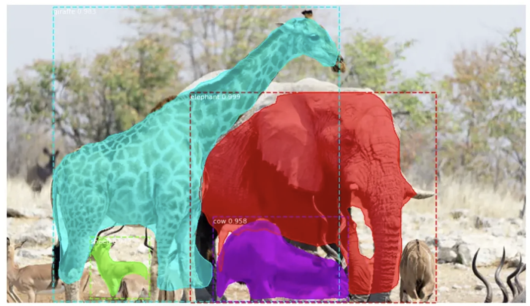
Instance Segmentation with Mask R-CNN

Mask R-CNN extends Faster R-CNN by adding a branch that outputs a pixel-level binary mask for each detected object. It provides exact spatial boundaries rather than simple rectangles. This is crucial for medical imagery, industrial defect segmentation, and scene understanding where object overlap makes bounding boxes ambiguous.

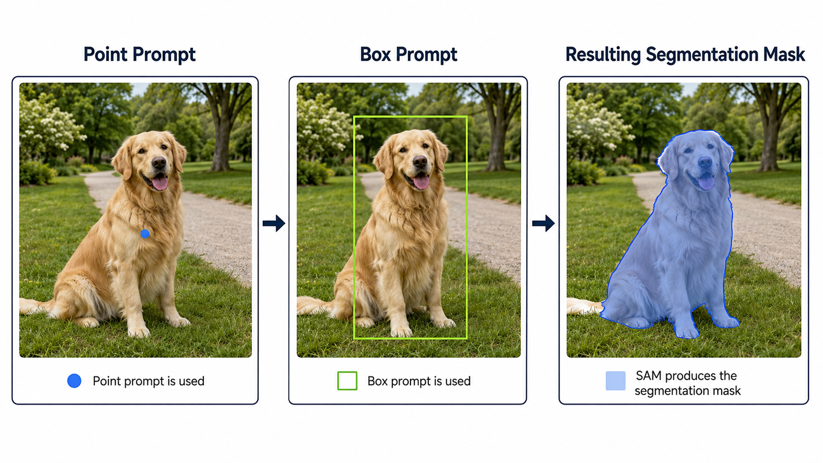
Segment Anything Model (SAM & SAM 2)

SAM is a promptable foundation model for segmentation. It can generate masks in a zero-shot manner based on user prompts:
• Point Prompt: User clicks a single point on an object; SAM generates its mask.
• Box Prompt: User draws a bounding box; SAM segments the object inside.
• Automatic Mask Generation: SAM segments every distinct object in the entire image.

SAM 2 extends this promptable capability to video, maintaining object mask consistency across consecutive frames despite motion and occlusion.

Note: SAM focuses on pixel boundaries but does not assign fixed class labels (e.g. "car") out of the box like standard supervised models.

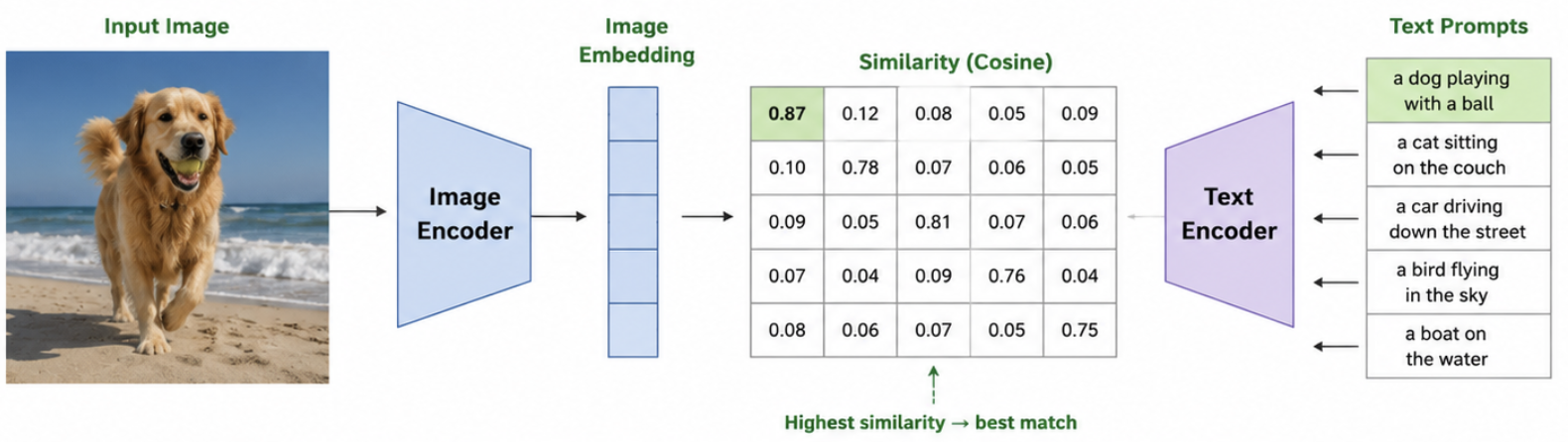
CLIP and Vision-Language Models

Shared Embedding Space

CLIP (Contrastive Language-Image Pretraining) maps images and natural language sentences into the same vector space.

How it works: An Image Encoder processes the image, and a Text Encoder processes text prompts (e.g., "a photo of a cat"). The model calculates the cosine similarity between the image embedding and multiple candidate text embeddings. The text embedding with the highest similarity indicates the predicted class. This enables zero-shot classification and semantic text-based image retrieval without training on fixed class labels.

For image embedding $\mathbf{v}$ and text embedding $\mathbf{t}_k$, CLIP compares normalized vectors: \[ s_k=\operatorname{cos}(\mathbf{v},\mathbf{t}_k) =\frac{\mathbf{v}^T\mathbf{t}_k}{\lVert\mathbf{v}\rVert_2\lVert\mathbf{t}_k\rVert_2}, \qquad p_k=\frac{\exp(s_k/T)}{\sum_j\exp(s_j/T)}. \] The highest similarity can support zero-shot classification over supplied prompts. CLIP itself is a dual-encoder similarity model, not a caption generator, although CLIP-like encoders can be components inside broader vision-language systems.

Segmentation Overlap Metrics

For predicted mask $P$ and ground-truth mask $G$: \[ \operatorname{IoU}(P,G)=\frac{|P\cap G|}{|P\cup G|},\qquad \operatorname{Dice}(P,G)=\frac{2|P\cap G|}{|P|+|G|}. \] For binary masks, $\operatorname{Dice}=2\operatorname{IoU}/(1+\operatorname{IoU})$. Both range from 0 (no overlap) to 1 (perfect overlap), assuming a nonempty union.

Model Type Comparisons

Model Type	Output Type	When to Use It
Object Detection	Bounding boxes + class labels	When object location is needed, but boundary shapes are not.
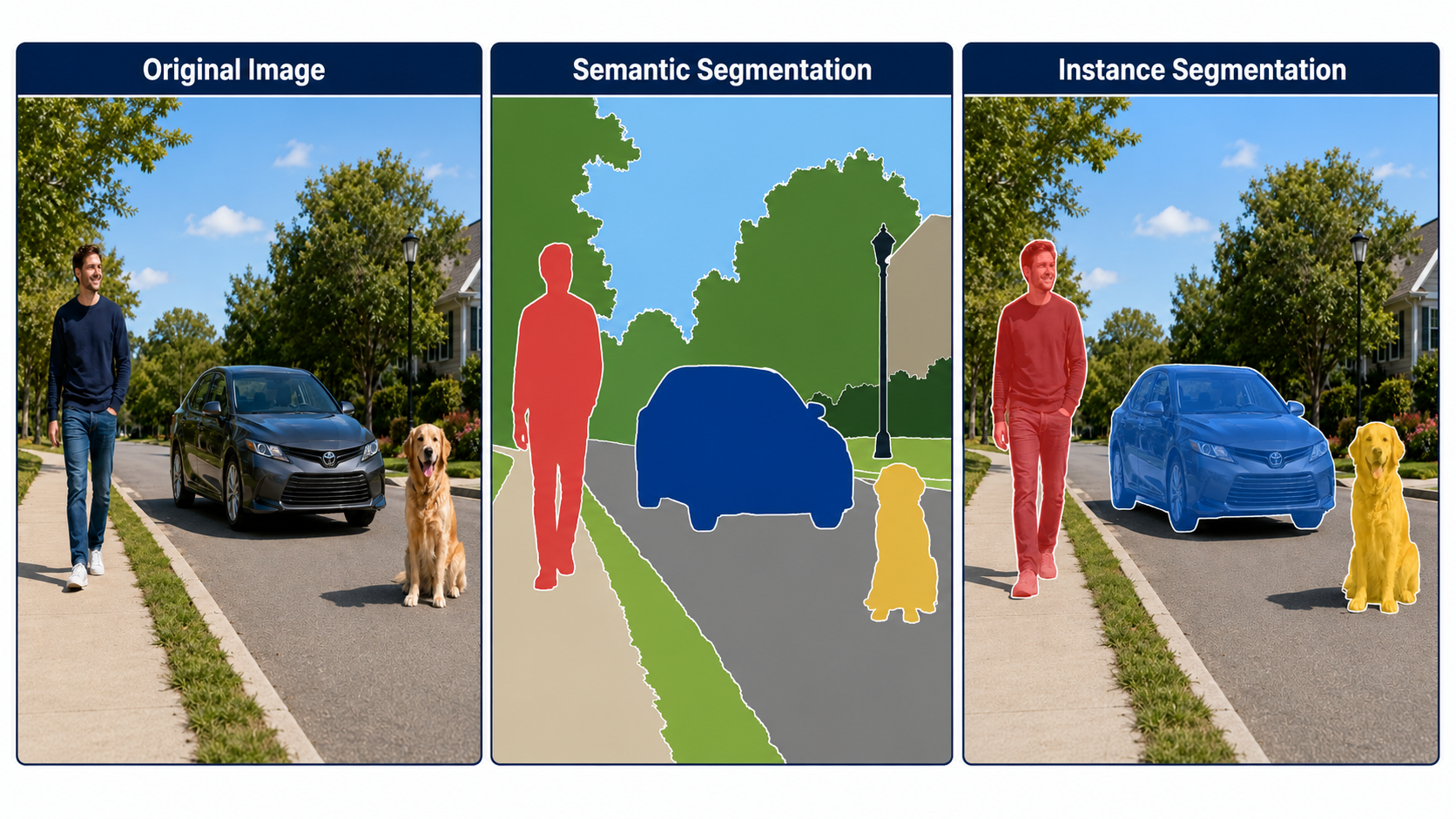
Semantic Segmentation	One class label per pixel (no instance separation)	When every pixel must be labeled (e.g. road vs. sidewalk vs. sky).
Instance Segmentation	Individual pixel mask per object instance	When you must separate different overlapping items of the same class.
Promptable Segmentation	Masks generated via clicks/boxes	For interactive labeling, editing, or unknown object masking.
Vision-Language Models	Image-text similarity vectors	For open-vocabulary recognition, captioning, or search.

Object Detection vs. Object Tracking

Detection

• Processes frames independently.

• Answers: Where are the objects in this single frame?

• No memory of past frames or object identities.

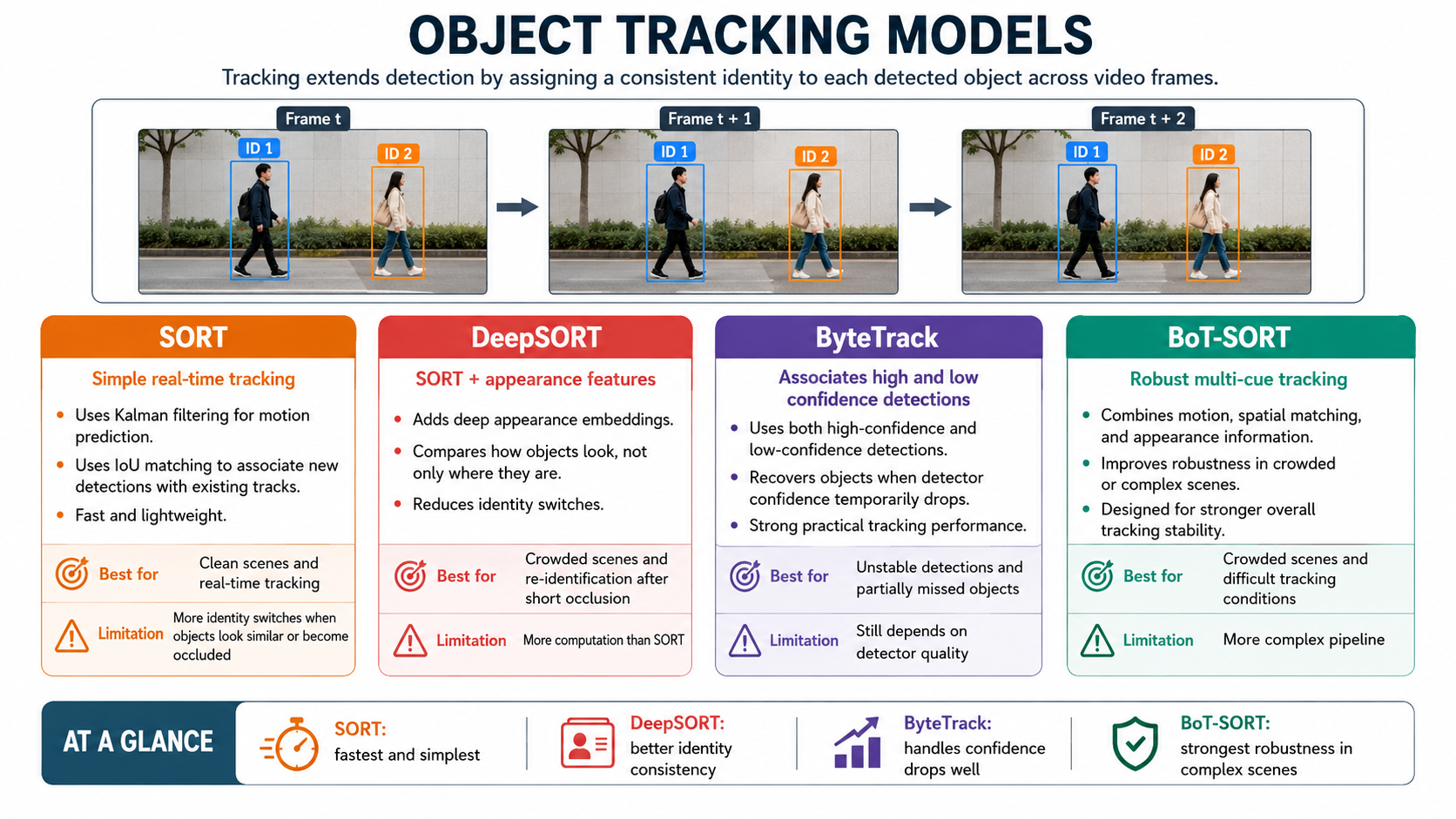
Tracking

• Links objects across consecutive frames.

• Answers: Which object in this frame is the same as in previous frames?

• Assigns and maintains a persistent Track ID.

Tracking-by-Detection Pipeline

1. Video Frames

→

2. Detector (e.g. YOLO)_{Find candidate boxes}

→

3. Data Association_{Link boxes across frames}

→

4. Track IDs_{Maintain consistent identities}

Common Tracking Algorithms

Model	Core Association Mechanism	Best For	Limitations
SORT	Kalman filtering (motion prediction) + IoU matching.	Fast, lightweight, real-time tracking in clear scenes.	High ID switches when objects overlap or are occluded.
DeepSORT	SORT + Deep Appearance Embeddings.	Crowded scenes; re-identifies objects after short occlusions.	Requires more computation to compute feature vectors.
ByteTrack	Associates both high and low confidence detections.	Unstable detections and recovering partially blocked objects.	Performance is heavily bound to detector quality.
BoT-SORT	Combines motion, spatial overlap, and appearance.	Highly complex tracking under difficult conditions.	Heavy computational pipeline.

Common Multi-Object Tracking Failures

ID Switch

Tracker swaps identities of two nearby or overlapping objects.

Track Fragmentation

One physical object's track is broken into multiple short tracks.

Occlusion Failure

Object gets temporarily hidden, and tracker loses it or assigns a new ID when it reappears.

Metrics across Vision Tasks

Task	Primary Metrics	Description
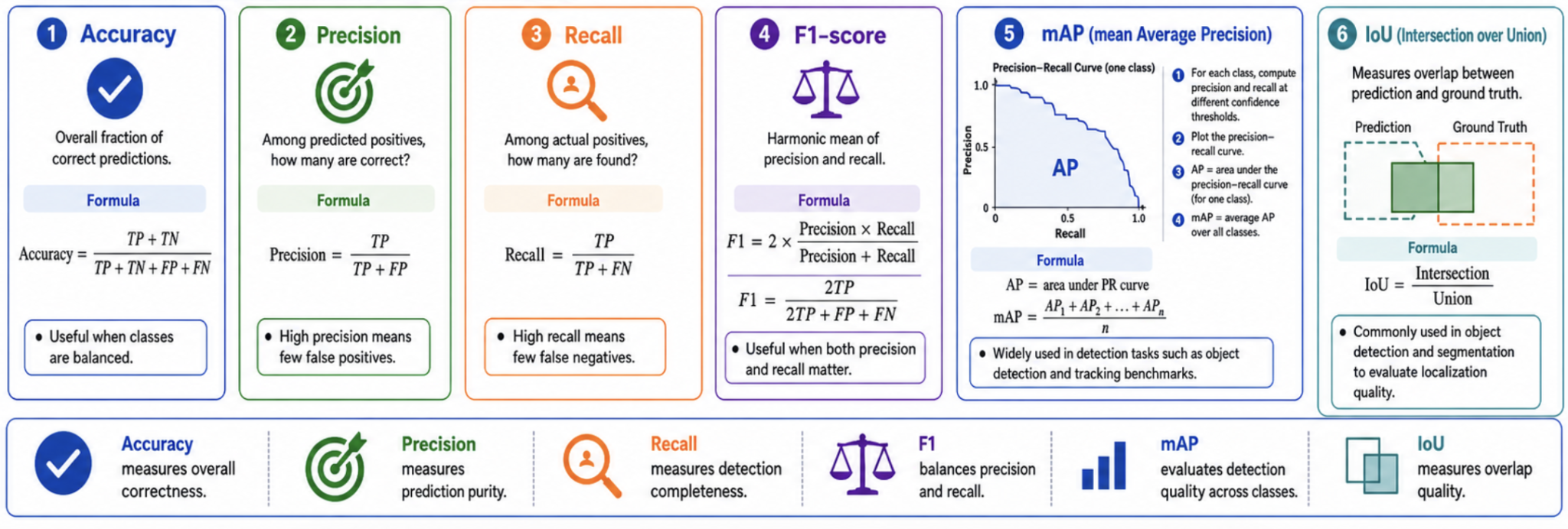
Classification	Accuracy, Precision, Recall, F1-score	Overall correctness, fraction of true positives among predictions, fraction of actual positives retrieved.
Detection	mAP (mean Average Precision), IoU	mAP calculates the area under the Precision-Recall curve averaged across all classes.
Segmentation	IoU (Jaccard Index), Dice Coefficient	Measures pixel-level overlap between predicted masks and ground-truth.
Tracking	ID Switches, MOTA, IDF1	Measures consistency of assigned track IDs over time.

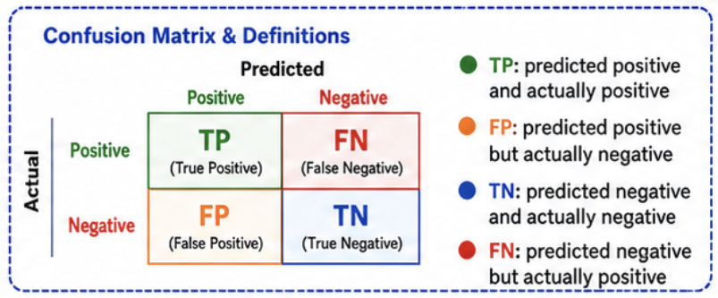
Classification and Detection Metrics

\[ \operatorname{Accuracy}=\frac{TP+TN}{TP+TN+FP+FN},\qquad \operatorname{Precision}=\frac{TP}{TP+FP},\qquad \operatorname{Recall}=\frac{TP}{TP+FN} \] \[ F_1=2\frac{\operatorname{Precision}\cdot\operatorname{Recall}} {\operatorname{Precision}+\operatorname{Recall}} =\frac{2TP}{2TP+FP+FN}. \] Undefined denominators require an explicit evaluation convention. Accuracy can be misleading for imbalanced classes, so always inspect per-class errors and the confusion matrix.

AP and mAP

Varying the confidence threshold traces a precision-recall curve. Conceptually, \[ AP_c=\int_0^1 P_c(R)\,dR,\qquad mAP=\frac{1}{C}\sum_{c=1}^{C}AP_c. \] Implementations use discrete/interpolated approximations. Always state the IoU protocol: $mAP@0.5$ is not the same as COCO-style $mAP@[0.5:0.95]$, which averages AP over IoU thresholds 0.50 through 0.95 in steps of 0.05.

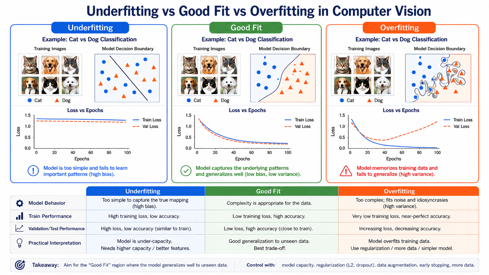
Underfitting vs. Overfitting in Computer Vision

Underfitting

Diagnosis: High train loss & high val loss.

Boundary: Too simple (linear) to separate data.

Fixes: Train longer, use larger model, better features.

Good Fit

Diagnosis: Low train loss & low val loss.

Boundary: Smooth, logical separation curve.

Fixes: Best model trade-off.

Overfitting

Diagnosis: Tiny train loss, high val loss.

Boundary: Highly squiggly, fits noise/points.

Fixes: Augmentation, dropout, early stopping, more data.

Deployment Considerations

• Edge Deployment (Mobile/Embedded): Requires low latency, low power, and small memory footprint. Compact models like MobileNet or YOLO-nano are preferred.
• Cloud Deployment (Server): Allows larger models (e.g. ResNet-152, large transformers) for high accuracy, but introduces network latency, server cost, and data privacy concerns.

Primary Technical References

• COCO official dataset site — dataset tasks and published statistics.
• DETR paper — end-to-end set prediction and bipartite matching without NMS.
• SAM 2 paper — promptable segmentation for images and videos with streaming memory.
• CLIP paper — contrastive image-text pretraining and zero-shot transfer.