Lecture 11: From Classical Vision to Deep Learning

Motivation & Recall

Recall: What Is Classification?

In classification, the model assigns an input sample to one of a predefined set of classes. A classifier can be understood as a model that learns decision boundaries separating samples from different classes. A simple model may learn a linear boundary, while a more powerful model may learn a non-linear boundary that bends around complex data distributions. In image classification, the decision is made from visual evidence in the image, such as shape, color, texture, edges, parts, and spatial arrangement. Example tasks include recognizing whether an image contains a cat, dog, car, zebra, tumor, or defective product.

The Classical Pipeline

Recall: Classical Recognition Pipeline

In a classical image recognition pipeline, the designer chooses the image features before training the classifier. Typical hand-crafted features include edges, corners, SIFT descriptors, HOG descriptors, color histograms, texture descriptors, and shape descriptors. In Bag of Visual Words (BOVW), local descriptors are extracted from images, clustered into a visual vocabulary, and converted into histograms. A classifier such as SVM then learns a boundary using these histograms. This pipeline can work well, but its performance depends strongly on the chosen descriptor, preprocessing choices, vocabulary size, and classifier settings.

Point Correspondences between Overlapping Images

A point correspondence means that a point in one image matches the same physical point in another image. For example, the corner of a window, the edge of a building, or a repeated texture point may appear in two overlapping images.

The usual correspondence pipeline is:

Detect feature points in the first and second images;
Describe each feature point using a descriptor;
Match descriptors between the two images;
Use the matched points to estimate the geometric transformation.

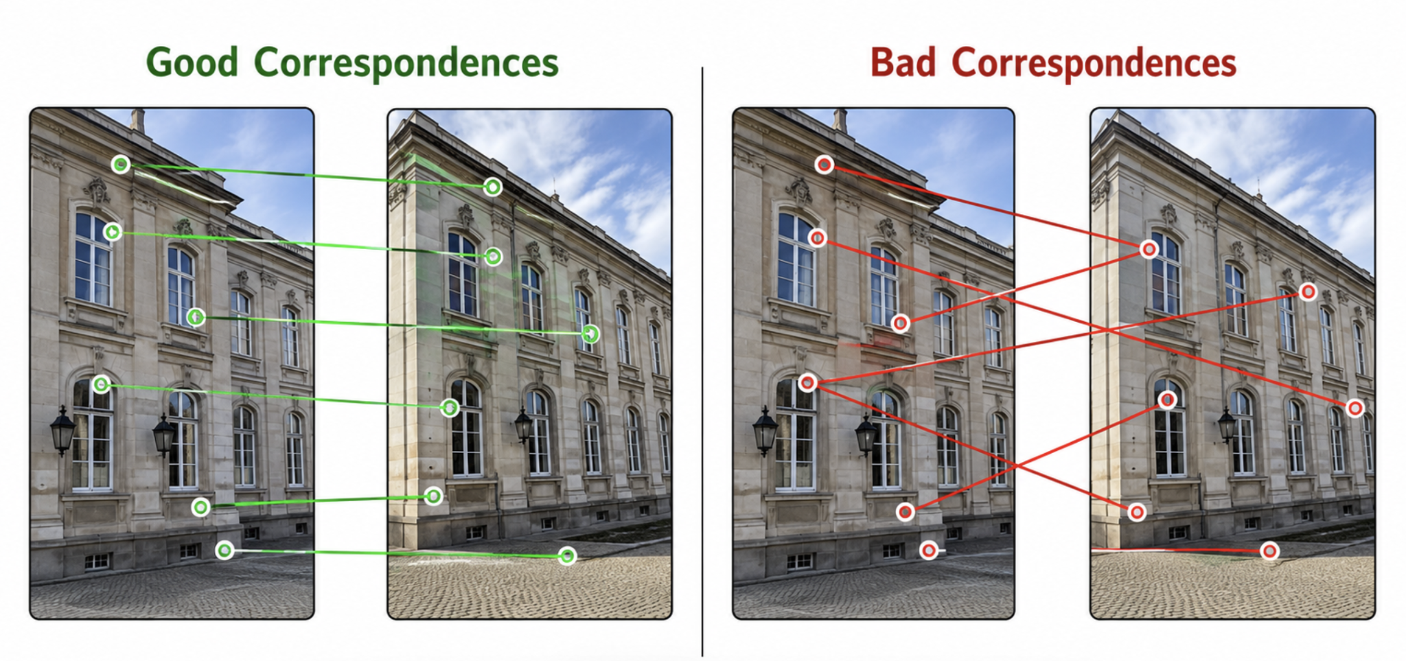
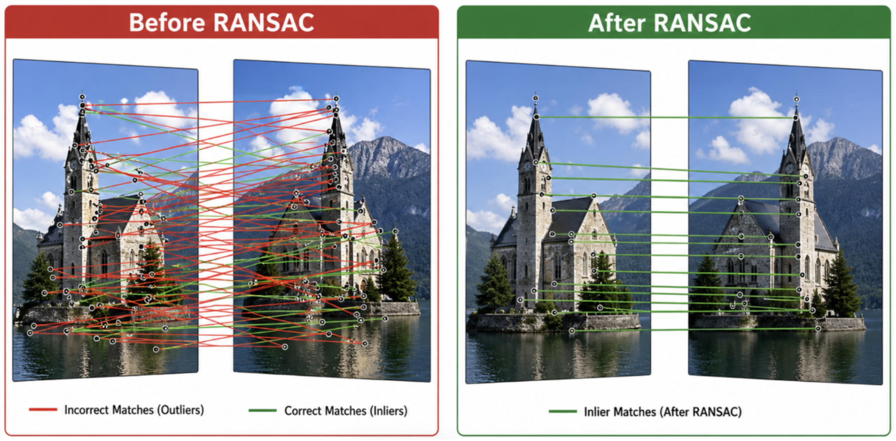
The Problem: Outliers in Feature Matching

In practice, feature matching is not perfect. Some matches are correct and follow the true image geometry (inliers), while other matches are wrong (outliers). Real image matching often produces outliers because of:

Repeated patterns, such as windows, bricks, or tiles;
Similar-looking object parts;
Noise and blur;
Occlusion;
Viewpoint and illumination changes;
Weak or ambiguous descriptors.

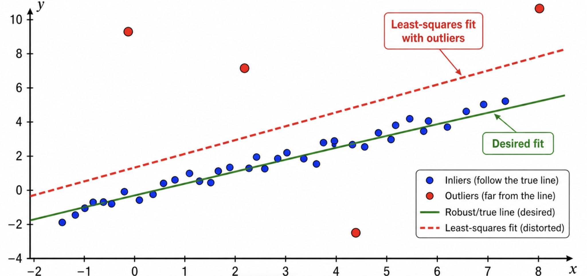
A normal least-squares fitting method can fail badly when outliers are present. This is because least squares tries to fit all points, including the wrong correspondences. Therefore, before estimating the final transformation, we need a method that can identify which matches are geometrically consistent. This is the main motivation for RANSAC.

Lecture Roadmap

Point Correspondence_{Matching & Outliers}

→

RANSAC_{Robust fitting & Homography}

→

Deep Learning Intro_{Classical vs CNN Features}

→

CNN Layer Details_{Convolutions, Padding, Stride}

→

Activation & Pooling_{ReLU, Downsampling, GAP}

→

Training & Augment_{Backpropagation & Generative AI}

What is RANSAC?

RANSAC: Random Sample Consensus

RANSAC is a robust model estimation algorithm used when the data contains both:

Inliers: Correct data points that agree with the true model.
Outliers: Incorrect data points that do not follow the model.

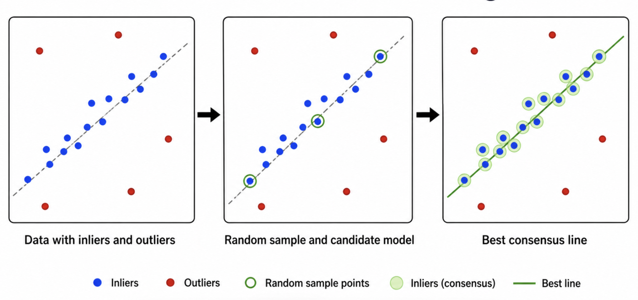
In computer vision, RANSAC is commonly used for: fitting lines or simple geometric models, estimating a homography, estimating a fundamental matrix, estimating camera pose, and image stitching / panorama creation. The key idea is to search for the model that is supported by the largest number of inliers. Instead of trusting all matches equally, RANSAC repeatedly tests random hypotheses and keeps the most consistent one.

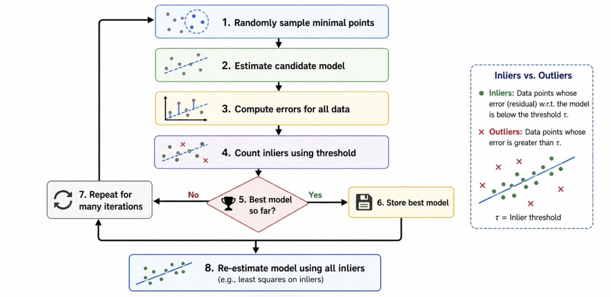
RANSAC Algorithm: Main Steps

Randomly sample: Select the minimum number of points needed to estimate the model (e.g., 2 points for a line, 4 points for a homography).

Compute model: Compute a candidate model from this random sample.

Test all points: Compute errors (residuals) for all other data points against the candidate model.

Count inliers: Count how many points fit the model within a chosen error threshold $\tau$ (residual $< \tau$). These agreeing points form the consensus set.

Update best: If this model has the largest number of inliers so far, store it. Repeat the loop for a predefined number of iterations.

Re-estimate: After all iterations, re-estimate the final model parameters using ALL inliers in the best consensus set (usually via least squares). This improves accuracy over using only the initial minimal sample.

Residuals, Consensus, and Required Iterations

For model $M$, residual function $r_i(M)$, and threshold $\tau$: \[ \mathcal{I}(M)=\{i:r_i(M)<\tau\},\qquad M^*=\arg\max_M |\mathcal{I}(M)|. \] If the estimated inlier fraction is $w$, a minimal sample contains $s$ points, and the desired probability of drawing at least one all-inlier sample is $p$, then \[ N=\left\lceil\frac{\log(1-p)}{\log(1-w^s)}\right\rceil. \]

Higher outlier rates or larger minimal samples require many more trials. RANSAC is probabilistically robust, not guaranteed to succeed. Degenerate samples must be rejected.

Core Terms

Model

The geometric relationship we want to estimate (e.g., line, homography, fundamental matrix).

Sample

A small, randomly selected subset of data points used to generate a candidate model.

Inlier & Outlier

An inlier has a residual below threshold $\tau$. An outlier has a residual above $\tau$.

Consensus Set

The set of all inliers supporting a candidate model.

Homography Mapping and Reprojection Error

In homogeneous coordinates, \[ \lambda\begin{bmatrix}u\\v\\1\end{bmatrix} =H\begin{bmatrix}x\\y\\1\end{bmatrix},\qquad H=\begin{bmatrix}h_{11}&h_{12}&h_{13}\\h_{21}&h_{22}&h_{23}\\h_{31}&h_{32}&h_{33}\end{bmatrix}. \] Let $(a,b,c)^T=H(x,y,1)^T$. The Euclidean projection and forward reprojection error are \[ \widehat{\mathbf{x}}'=\left(\frac{a}{c},\frac{b}{c}\right)^T,\qquad e=\lVert\mathbf{x}'-\widehat{\mathbf{x}}'\rVert_2. 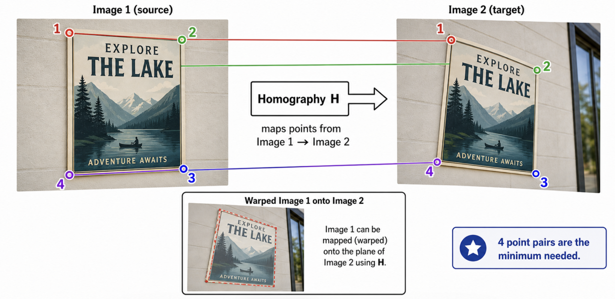\] Four correspondences are the algebraic minimum because $H$ has 8 degrees of freedom, but no three sampled source or destination points may be collinear. For accurate estimation, normalized DLT and a symmetric transfer error are often preferred.

Homography Estimation using RANSAC

Homography Matrix ($H$)

A homography maps points from one image plane to another image plane. Homography estimation is important in: panorama stitching, image alignment, document rectification, planar object localization, and camera rotation-based mosaics.

The RANSAC loop for homography estimation is:

Randomly select 4 point correspondences;
Compute a candidate homography matrix $H$;
Project points using $H$;
Count matches whose projection error is below a threshold;
Keep the homography with the largest inlier set;
Recompute $H$ using all inliers.

RANSAC is critical here because even a single bad correspondence can corrupt the homography if not rejected.

Why Four Points?

A projective transformation (homography) is represented by a $3 \times 3$ matrix. Since the matrix is defined up to scale, it has 8 degrees of freedom.

Each point correspondence provides 2 independent constraints:
• One constraint for the x-coordinate
• One constraint for the y-coordinate

Therefore, we need at least 4 points:
$$4 \text{ points} \times 2 \text{ constraints/point} = 8 \text{ constraints}$$

Error Threshold Selection

The threshold $\tau$ controls the strictness of the inlier decision:

• A very small threshold may reject correct matches due to noise.

• A very large threshold may accept wrong matches as inliers.

Choosing a reasonable threshold is essential for stable model estimation.

RANSAC Strengths and Limitations

Strengths

✔ Can tolerate high outlier percentages when the inlier model is dominant enough and the iteration budget is sufficient.
✔ Conceptually simple and mathematically clear.
✔ Applicable to many different geometric models (lines, circles, homographies, fundamental matrices).
✔ Cleans feature matches before final calculation.

Limitations

✗ Randomized: results can vary between runs on the same data.
✗ Computational cost: may require many iterations when the outlier ratio is high.
✗ Dependent on threshold parameters.
✗ Assumes enough inliers exist to support the correct model.
✗ Can fail when multiple different models are present in the same data.

RANSAC vs. Hough Transform

Property	Hough Transform	RANSAC
Strategy	Voting space (parameter bins)	Random sampling and consensus
Parameterization	Quantized accumulator space	Mathematical equations fit to samples
Complexity	Grows exponentially with dimensions	Depends on outlier ratio & model dimensions
Typical Uses	Simple shapes: lines, circles, ellipses	Homographies, fundamental matrices, camera pose
Noise / Multi-model	Can find multiple peaks simultaneously	Usually fits one dominant model at a time

RANSAC in the Image Correspondence Pipeline

1. Detect Keypoints

→

2. Compute Descriptors

→

3. Match Descriptors

→

4. RANSAC (Reject Outliers)

→

5. Estimate Homography

→

6. Image Warping & Blending

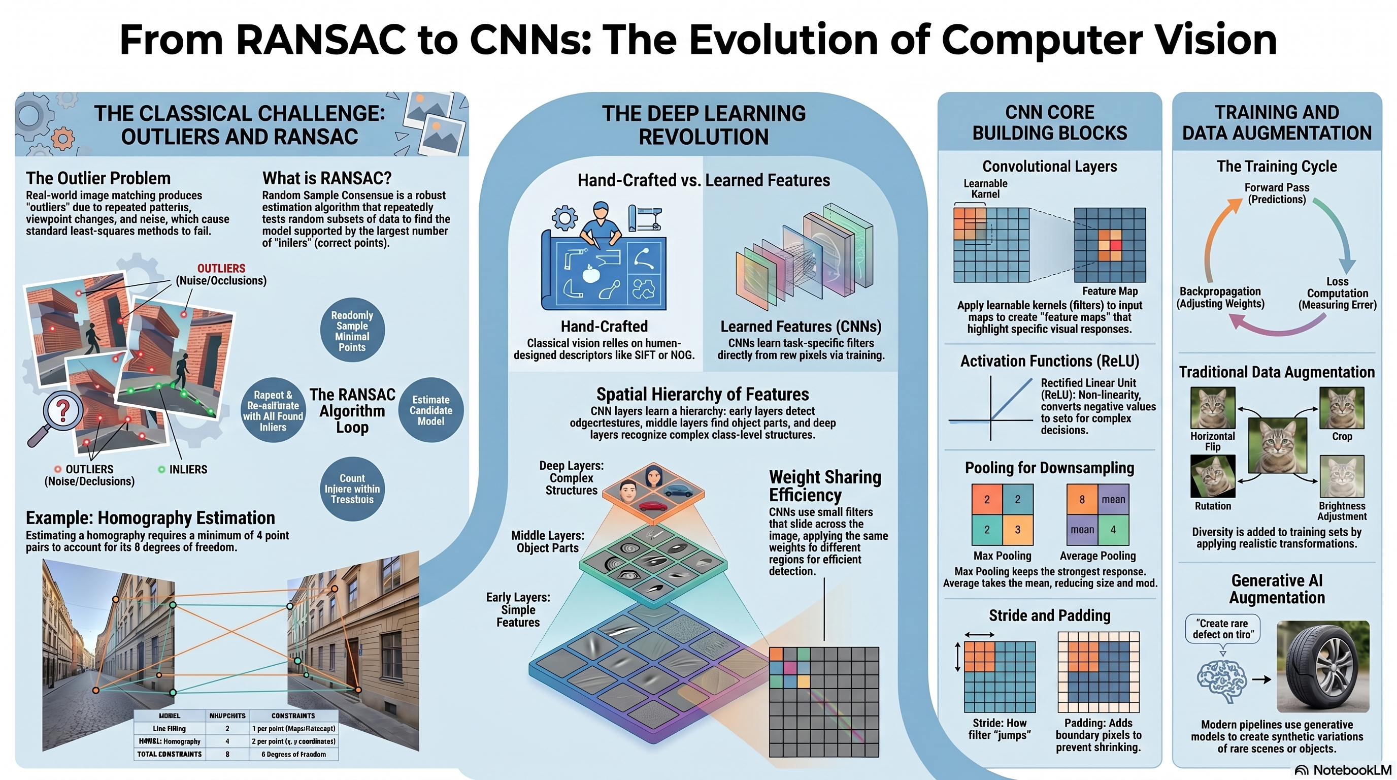
From RANSAC to Deep Learning

RANSAC is a strong example of a classical computer vision method. It depends on explicitly designed steps: feature detection, descriptor extraction, feature matching, geometric model estimation, and outlier rejection. These classical pipelines are powerful, but they require careful design and depend heavily on the quality of the hand-crafted features. Convolutional Neural Networks (CNNs) introduce a different approach. Instead of manually designing all feature extraction steps, CNNs learn useful visual filters directly from training images.

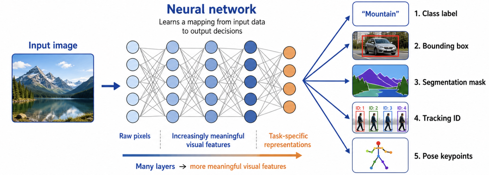
Neural Networks in Computer Vision

A neural network is a machine learning model that learns a mapping between input data and output decisions using layers of connected computational units called neurons. In computer vision, the input is usually an image, and the output may be:
1. Class label (classification)
2. Bounding box (object detection)
3. Segmentation mask (semantic/instance segmentation)
4. Tracking identity (object tracking)
5. Pose keypoint (pose estimation)

The model is called deep when it contains many layers that gradually transform raw pixels into more meaningful visual representations. The key is that the network learns statistical visual patterns from many examples, rather than relying on human engineering.

Classical Features vs. CNN Features

Classical Features (Hand-Crafted)

• The user decides what the feature means (e.g., corner strength, edge orientation, local gradient pattern).

• Hand-crafted descriptors (SIFT, HOG, LBP) extract features first, then a separate classifier (SVM, Random Forest) makes decisions.

CNN Features (Learned)

• The network learns useful filters during training. Feature extraction and classification are combined into one unified, trainable model.

• Filters adapt to the training dataset through backpropagation to minimize predictive loss.

Feature Hierarchy in Deep Networks

Early Layers

Respond to simple structures

Edges & boundary contrasts

Basic colors & textures

Middle Layers

Combine simple patterns

Corners & repeated shapes

Object parts & texture layouts

Deep Layers

Class-specific features

Faces, wheels, animal parts

Complex semantic shapes

Why CNNs Are Crucial for Vision

Images are not random vectors; nearby pixels are strongly related because visual objects have spatial structure. A CNN exploits this through:

Local Connectivity: Small filters slide across the image, focusing on small spatial neighborhoods.
Weight Sharing: The same filter is applied at all positions. This allows the network to detect a visual pattern wherever it appears (translation invariance/equivalence) and makes it much more parameter-efficient than fully connected networks.

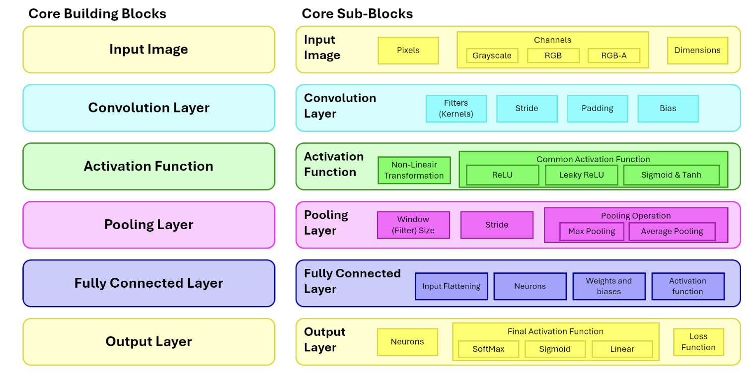
Basic CNN Architecture

CNN Pipeline: From Image to Prediction

A typical CNN contains a feature extraction part followed by a decision-making part.

Feature Extraction: Repeated blocks of Convolutions, Activations (like ReLU), and Pooling.
Decision-making: Flattening / GAP, Fully connected (Dense) layers, and Softmax / Sigmoid output.

Input Image_{Pixels & Channels}

→

Convolution_{Apply filters}

→

ReLU_{Non-linearity}

→

Pooling_Downsampling

→

Flatten / GAP_{Vector conversion}

→

Dense Layers_{Feature combination}

→

Output_{Probabilities / Scores}

The Convolutional Layer

How Convolutions Work

A convolutional layer applies trainable filters to an input. Each filter is a small matrix called a kernel (e.g., $3 \times 3$, $5 \times 5$, $7 \times 7$). The kernel slides over the image and computes a weighted sum at each spatial location. The output produced by one filter is a feature map (or response map). If a layer has 32 filters, it outputs 32 feature maps.

Unlike classical filters (Sobel, Laplacian) which have fixed, designer-specified values, CNN filters are initialized randomly and updated during training through backpropagation.

Kernel Size and Receptive Field

• Kernel Size: Controls the local neighborhood examined at each step. $3 \times 3$ is popular because it is parameter-efficient and can be stacked to build larger receptive fields.
• Receptive Field: The region of the original input image that influences a specific neuron in a deeper feature map. Deeper layers have larger receptive fields, allowing them to comprehend larger object structures.

Multi-Channel Convolution and Parameter Count

For input $X\in\mathbb{R}^{H\times W\times C_{in}}$, output channel $k$, and cross-correlation kernel $W^{(k)}\in\mathbb{R}^{F_h\times F_w\times C_{in}}$: \[ Y_{i,j,k}=b_k+\sum_{u=0}^{F_h-1}\sum_{v=0}^{F_w-1} \sum_{c=1}^{C_{in}}W^{(k)}_{u,v,c}\,X_{iS_h+u-P_h,\,jS_w+v-P_w,\,c}. \] With $C_{out}$ filters, the trainable parameter count is \[ (F_hF_wC_{in}+1)C_{out}, \] where the $+1$ is one bias per output channel. One filter spans all input channels and produces one output feature map.

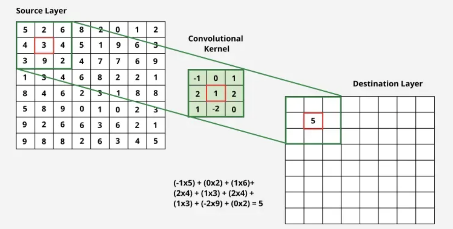
Worked 3x3 Kernel Example from the Lecture

\[ X=\begin{bmatrix}5&2&6\\4&3&4\\3&9&2\end{bmatrix},\qquad K=\begin{bmatrix}-1&0&1\\2&1&2\\1&-2&0\end{bmatrix} \] Using the unflipped CNN operation (cross-correlation), \[ \sum X\odot K=-5+0+6+8+3+8+3-18+0=\boxed{5}. \]

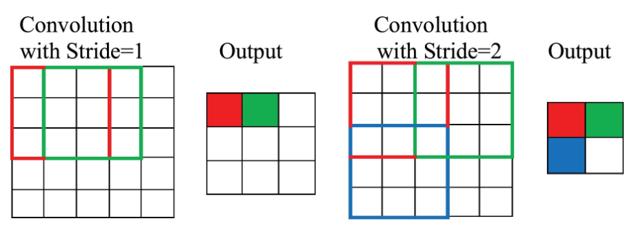
Stride and Output Size Formula

Stride & Spatial Calculations

Stride ($S$) determines how many pixels the kernel moves each time it slides. Stride 1 moves 1 pixel at a time. Stride 2 jumps 2 pixels, downsampling the output. Larger strides reduce computation but may lose fine details.

If the input image has spatial size $N \times N$, the kernel has size $F \times F$, the stride is $S$, and the padding is $P$, the output spatial size is:

\[ H_{out}=\left\lfloor\frac{H+2P_h-D_h(F_h-1)-1}{S_h}\right\rfloor+1, \qquad W_{out}=\left\lfloor\frac{W+2P_w-D_w(F_w-1)-1}{S_w}\right\rfloor+1. \] For dilation $D_h=D_w=1$ and square inputs, this reduces to \[ N_{out}=\left\lfloor\frac{N-F+2P}{S}\right\rfloor+1. \]

Example: For $N=7$, $F=3$, Stride $S=2$, and Padding $P=0$:
$\text{Output Size} = \lfloor(7 - 3) / 2\rfloor + 1 = 2 + 1 = 3$. The output feature map is $3 \times 3$.

Receptive Field Growth

Let $r_l$ be receptive-field size and $j_l$ the spacing (“jump”) between adjacent layer-$l$ features in input pixels. Starting with $r_0=j_0=1$: \[ j_l=j_{l-1}S_l,\qquad r_l=r_{l-1}+(F_l-1)D_lj_{l-1}. \] Thus, two stride-1 $3\times3$ layers have a $5\times5$ receptive field while using fewer parameters and adding an extra nonlinearity compared with one $5\times5$ layer.

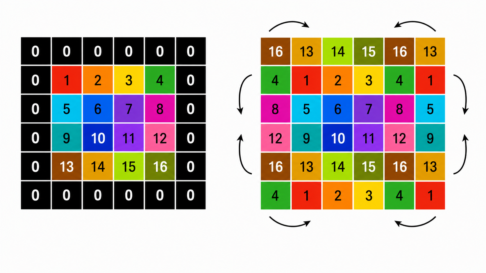
Padding: Zero vs. Circular

Zero Padding

Adds extra boundary pixels filled with zeros. Allows the filter to process edge and corner pixels fairly. With $F=3$, Stride $S=1$, adding $P=1$ padding keeps the output size identical to the input size.

Circular Padding

Fills boundary cells by wrapping pixels from the opposite side of the image:
• Left boundary is filled using right-side pixels.
• Right boundary is filled using left-side pixels.
• Top boundary is filled using bottom pixels.
• Bottom boundary is filled using top pixels.

Convolution vs. Cross-Correlation

In mathematics, convolution requires flipping the kernel horizontally and vertically before sliding it. In cross-correlation, the kernel is applied directly without flipping.

Most deep learning libraries (like PyTorch, TensorFlow) actually implement cross-correlation but call it convolution. In practice, this does not affect training because the filter values are learned anyway; the network simply learns flipped weights if necessary.

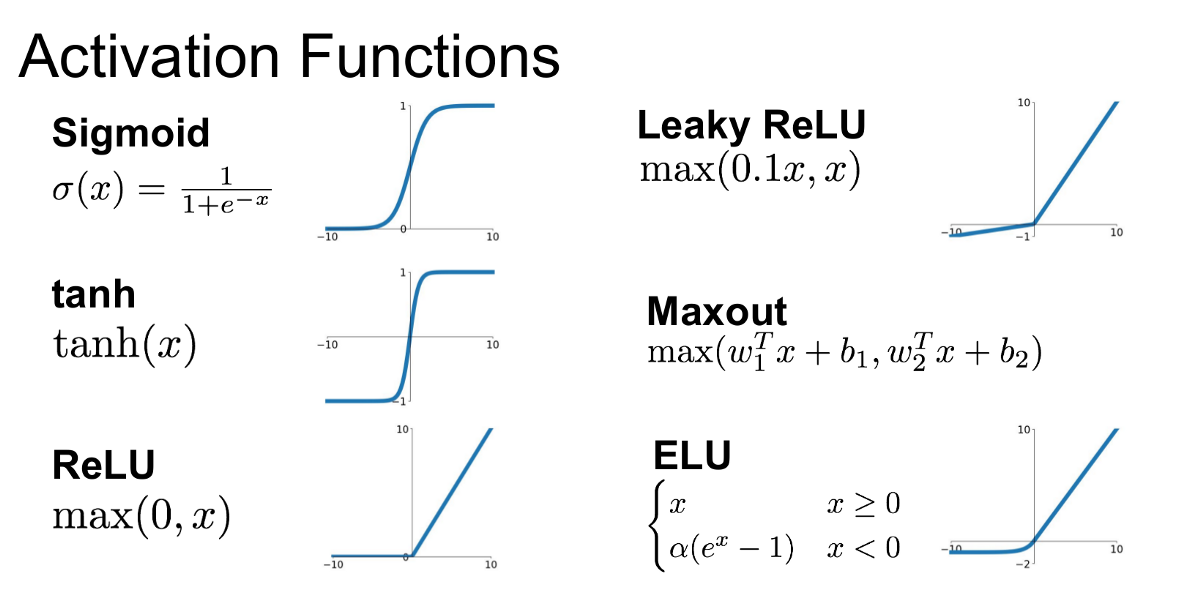
Why Do We Need Activation Functions?

A convolutional layer alone is a linear weighted operation. Stacking multiple linear layers would still only represent a single linear transformation. An activation function introduces non-linearity, allowing the model to learn complex decision boundaries. It operates element-wise, keeping the spatial dimensions identical.

Common Activation Functions

Function	Equation	Characteristics
ReLU	$f(x) = \max(0, x)$	Simplest, computationally efficient, creates sparse activation maps. Prevents vanishing gradients in positive regions.
Leaky ReLU	$f(x) = \max(0.1x, x)$	Allows a small gradient for negative inputs to prevent "dying ReLU" issues.
Sigmoid	$\sigma(x) = 1 / (1 + e^{-x})$	Outputs range $(0, 1)$. Good for binary classification / multi-label output. Can suffer from vanishing gradients.
Tanh	$\tanh(x)$	Outputs range $(-1, 1)$. Zero-centered.
ELU	$x$ if $x \ge 0$, else $\alpha(e^x - 1)$	Smooth curve for negative values.
Maxout	$\max(w_1^T x + b_1, w_2^T x + b_2)$	Generalizes ReLU and Leaky ReLU.

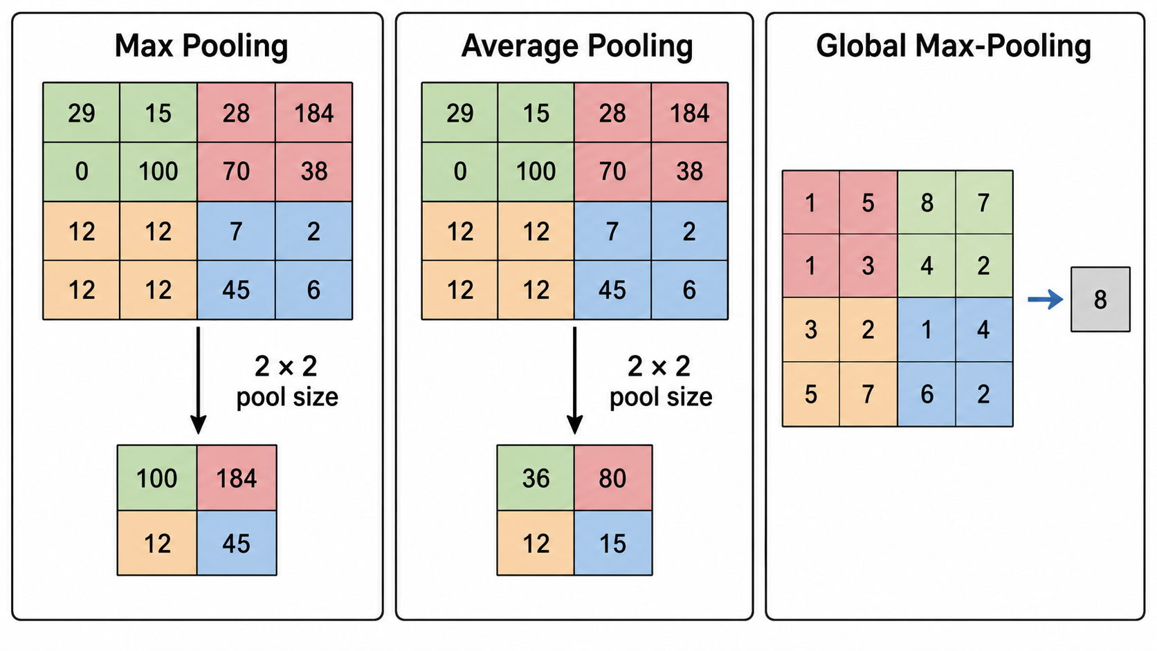
Pooling Layers

Pooling is a downsampling operation that reduces spatial dimensions to decrease computation and parameters. Pooling does NOT contain learnable weights; it performs fixed aggregations.

Max Pooling

Keeps the maximum value in each pooling window. Useful for preserving the strongest detected feature in that region.

Average Pooling

Computes the average value of the window. Smooths out features.

Global Average Pooling (GAP)

Reduces the entire feature map ($H \times W$) to a single value by averaging all pixels. Greatly reduces parameters before fully connected layers.

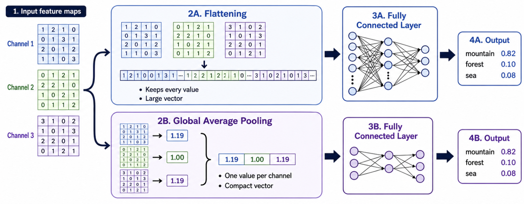
Decision Layer Transitions: Flattening vs. GAP

Flattening

Converts $H \times W \times C$ feature maps into a single 1D vector of size $(H \cdot W \cdot C)$. Passes all spatial values directly to dense layers.
Con: Leads to very large fully connected layers, high parameter counts, and higher risk of overfitting.

Global Average Pooling (GAP)

Averages each channel's feature map, outputting a vector of size $1 \times 1 \times C$.
Pro: Drastically reduces parameter count, improves generalization, and acts as a structural regularizer.

Output Activations: Softmax vs. Sigmoid

• Softmax: Converts raw class scores (logits) into probabilities that sum to 1. Used in multi-class classification (where each image belongs to exactly one class).
• Sigmoid: Outputs independent probabilities for each class. Used in multi-label classification (where an image can contain multiple classes, e.g., both "dog" and "car").

For logits $\mathbf{z}$ and $C$ mutually exclusive classes, \[ p_k=\operatorname{softmax}(\mathbf{z})_k= \frac{e^{z_k}}{\sum_{j=1}^{C}e^{z_j}},\qquad \sum_{k=1}^{C}p_k=1. \] With one-hot target $\mathbf{y}$, categorical cross-entropy is \[ \mathcal{L}_{CE}=-\sum_{k=1}^{C}y_k\log p_k=-\log p_{\text{true}}. \] For independent multi-label targets, use one sigmoid per class and binary cross-entropy: \[ \sigma(z_k)=\frac{1}{1+e^{-z_k}},\qquad \mathcal{L}_{BCE}=-\sum_k\left[y_k\log p_k+(1-y_k)\log(1-p_k)\right]. \]

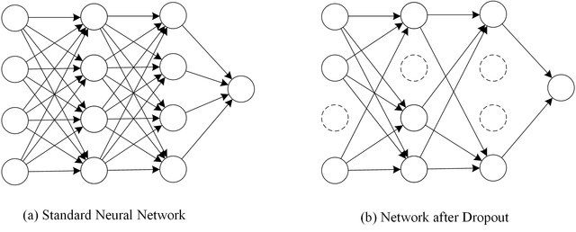
Regularization: Dropout & Overfitting

Overfitting occurs when a model performs exceptionally on training data but generalizes poorly to validation data.

Dropout is a regularization technique that randomly deactivates (sets to zero) a percentage of neurons during each training step. This prevents co-dependency among neurons, encouraging the network to learn robust, distributed representations.

With inverted dropout, mask $m_i\sim\operatorname{Bernoulli}(q)$ and keep probability $q=1-p_{drop}$: \[ \widetilde{a}_i=\frac{m_i}{q}a_i\quad\text{during training},\qquad \widetilde{a}_i=a_i\quad\text{during inference}. \] The $1/q$ scaling preserves the expected activation. Dropout is disabled at inference.

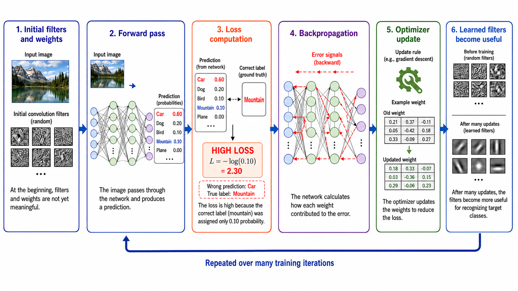
How CNN Training Works

Initialization: Filters and weights are initialized with random or pre-trained values.

Forward Pass: An image passes through the layers, outputting class scores / probabilities.

Loss Computation: The output prediction is compared to the ground truth label using a loss function (e.g., Categorical Cross-Entropy). A high loss means the model was confident in the wrong class.

Backpropagation: The model calculates the gradients of the loss with respect to every weight using the chain rule, showing how each filter parameter contributed to the error.

Optimizer Update: An optimizer (e.g., Adam, SGD) updates the weights in the opposite direction of the gradients to reduce the loss in future passes.

Loop: The process repeats over many training iterations until the filters learn useful, discriminative visual patterns.

Gradient-Based Weight Update

For learning rate $\eta$, a basic stochastic-gradient update is \[ \theta_{t+1}=\theta_t-\eta\nabla_{\theta}\mathcal{L}_{batch}(\theta_t). \] Backpropagation computes $\nabla_{\theta}\mathcal{L}$ efficiently by repeatedly applying the chain rule through the computational graph. Adam and momentum SGD modify the update using running gradient statistics, but still seek to reduce the loss.

Samples, Batches, and Epochs

Sample

A single training example (e.g., one image and its corresponding label).

Batch

A small group of samples processed together. Weights are updated after each batch.

Epoch

One complete pass through the entire training dataset.

For $N$ training samples and batch size $B$, batches per epoch are \[ \left\lceil\frac{N}{B}\right\rceil. \] For the lecture example, $N=200$ and $B=5$, so one epoch contains $40$ updates; $1000$ epochs contain $40{,}000$ batch updates.

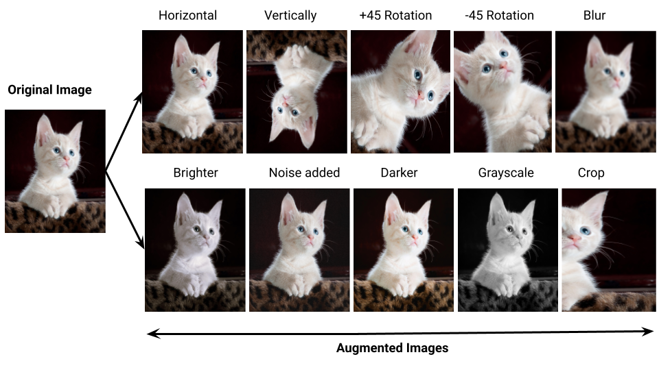
Data Augmentation

Artificially Increasing Dataset Diversity

When training data is limited, the model can easily overfit. Data augmentation applies random transformations to images to create synthetic training samples.

Geometric Transformations:
• Horizontal Flipping: Great for classifying animals/objects, but bad for digits (e.g., 6 vs 9) or traffic signs where direction matters.
• Rotations, Translation, Zooming, Cropping, and Stretching.

Appearance Transformations:
• Brightness, Contrast, Color changes, Blur, and Sharpness.

Advanced Methods:
• Random Erasing: Simulates occlusions.
• CutMix / MixUp: Blends images together.

Generative AI for Data Augmentation

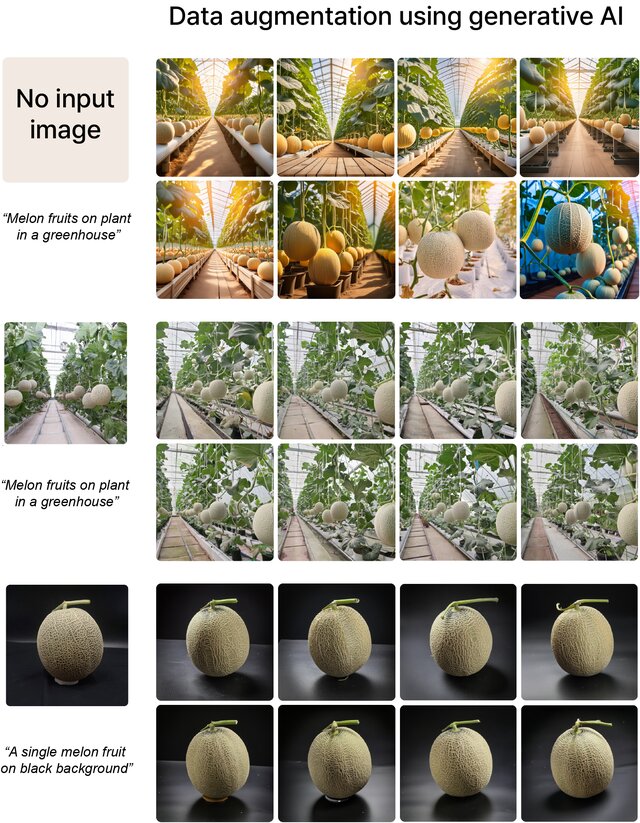
Generative AI (like Diffusion Models) can create realistic new images when training data is small, imbalanced, or missing key variations.

• Text-to-Image: Generating images purely from text descriptions.
• Image-to-Image (Scene): Providing a base scene and using prompts to change the background or style.
• Image-to-Image (Object): Generating variations of a single object on different backgrounds.

Caution: Generated images must be used carefully. They can introduce unrealistic details, incorrect shapes, incorrect labels, or digital artifacts, which could lead to poor generalization on real-world test data.