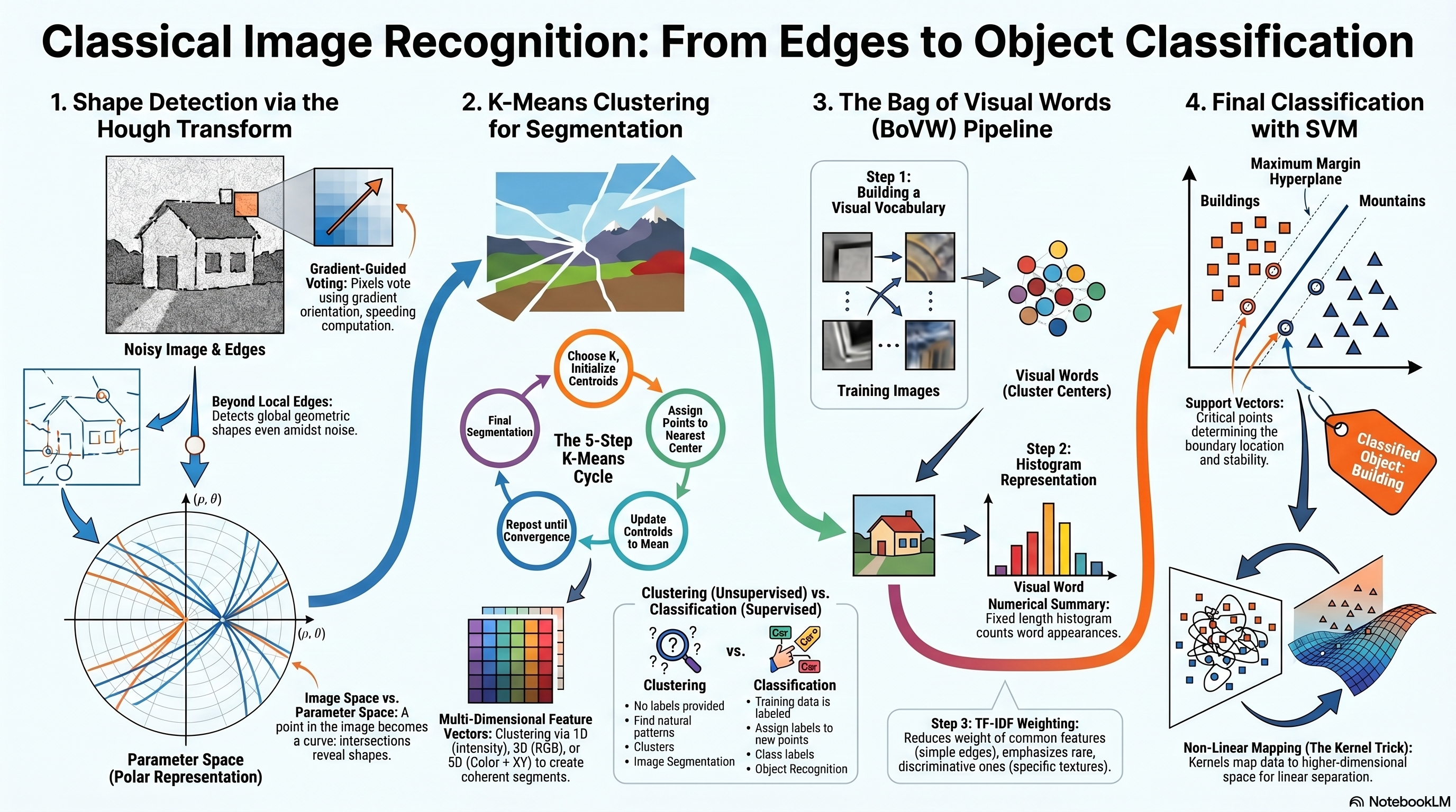
So far in the course, we have studied several techniques that allow us to detect local image features, such as edges, corners, and keypoints. We also learned how to construct descriptors that represent these features numerically. However, detecting individual features alone is not sufficient for understanding the global structure of objects in an image. Instead, we often need to detect geometric shapes such as straight lines, circles, curves, and object templates. The Hough Transform is a classical technique that allows us to detect such shapes even in the presence of noise, missing edge segments, multiple overlapping structures, and cluttered backgrounds. In this lecture, we focus primarily on line detection using the Hough Transform.
Why the Hough Transform Is Needed
Even after edge detection produces an edge map, detecting complete geometric structures is not straightforward because: detected edges may contain extra points from clutter, multiple different lines may exist in the same image, only partial segments of a line may be detected, edge measurements may be corrupted by noise, and gradient orientations may be inaccurate. Therefore, we need a robust method that recovers complete line structures from incomplete observations. The Hough Transform provides such a solution.
What the Hough Transform Can Detect
Straight Lines
2 parameters: slope & intercept
Or: ρ and θ (polar)
Primary focus of Lec 10
Circles
3 parameters: a, b, r
2D if r known; 3D if unknown
Extended Hough
Ellipses
Center, axes, orientation
5-parameter space
Higher-D Hough
Arbitrary Shapes
Template + R-table
Generalized Hough Transform
Any parametric shape
Key Advantages of the Hough Transform
Robust to Noise
Voting averages out noise
False edge pixels contribute few votes
True lines accumulate many votes
Handles Partial Lines
Works with incomplete edge segments
Each edge pixel votes independently
No need for connected contours
Multiple Detections
Finds multiple lines simultaneously
Each line becomes a separate peak
Handles overlapping structures
Lecture Roadmap
Edge DetectionRecap: scale-space
→
Hough BasicsLine parameters, image→param space
→
Polar Formρ, θ representation
→
AlgorithmVoting & accumulator
→
Circles & ExtensionsCircle, generalized Hough
Single-Scale vs Multi-Scale Edge Detection
Edge detection results depend strongly on the choice of the Gaussian smoothing parameter σ. In single-scale edge detection, the image is filtered using only one value of σ. A small σ detects fine details but keeps noise. A large σ removes noise but may blur important edges. Therefore, selecting one fixed scale creates a trade-off between accuracy and robustness. In multi-scale edge detection, the image is filtered using multiple values of σ simultaneously.
Small σ (fine scale)
Fine details preserved
Noise remains present
Detects thin, fine-texture edges
Medium σ
Balance of detail and noise
Object boundaries clearer
Detects structural boundaries
Large σ (coarse scale)
Heavy smoothing applied
Only strong edges remain
Detects dominant structural edges
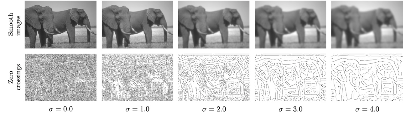
Edge Detection Across Scale-Space
How edge detection changes as σ increases
Each column in a scale-space diagram represents edge detection performed at a single scale using one specific value of σ. Therefore, one column = single-scale edge detection, and all columns together = multi-scale edge detection. When σ = 0, almost no smoothing is applied and many detected edges correspond to noise and fine texture. When σ increases (e.g., 1.0 and 2.0), small noisy edges disappear and meaningful object boundaries become clearer. When σ becomes large (e.g., 3.0 and 4.0), only strong structural edges remain and fine details are removed. This demonstrates the idea of scale-space representation.
Stability Across Scales
If an edge appears only at a very small scale, it may correspond to noise, texture, or a fine detail. If an edge remains visible across several scales, it is more likely to be a strong and meaningful structural edge. Therefore, stable edges across multiple scales are usually more reliable than edges that appear only at one scale.
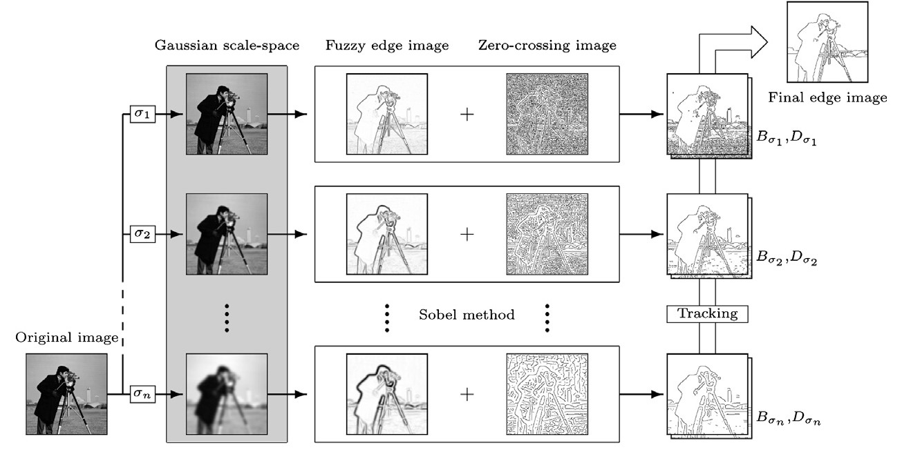
Multi-Scale Edge Detection Pipeline
1
Original image: May contain noise and fine texture details that interfere with accurate edge detection.
2
Gaussian scale-space filtering with different values of σ. Small σ preserves fine details and detects thin edges. Large σ suppresses noise and emphasizes stronger structural edges.
3
Gradient-based edge estimation: At each scale, a gradient-based method such as Sobel is used to estimate edge strength and produce a fuzzy edge image.
4
Zero-crossing image: Computed using a second-derivative response to help localize edge positions more precisely. The fuzzy edge image and zero-crossing image are combined to obtain candidate edges at each scale.
5
Edge tracking: Edges from different scales are connected through a tracking stage to produce the final edge image.
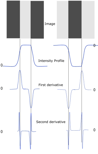
What Does Zero-Crossing Mean in Edge Detection?
Second-derivative edge localization
Zero-crossings are associated with second-derivative edge detection methods such as the Laplacian or Laplacian of Gaussian (LoG). A zero-crossing occurs when the filtered signal changes sign from positive to negative or from negative to positive. This sign change indicates a location where the image intensity curvature switches direction. Such locations correspond to edge boundaries in the image. The key idea comes from the second-derivative property: the first derivative detects edge strength and the second derivative detects edge position precisely.
First derivative → detects WHERE intensity changes rapidly (edge strength)
Second derivative → detects WHERE sign changes (edge position / zero-crossing)
Zero-crossing: the signal goes from (+) to (−) or (−) to (+)
This sign change marks a precise edge boundary.
LoG zero-crossings are commonly used for precise edge localization.
Edges detected in this way are sharper than gradient-magnitude thresholding.
Motivation for the Hough Transform
The final output of multi-scale edge detection is a refined edge map that balances noise suppression, edge localization accuracy, and detection of both fine and strong edges. However, detecting complete lines from edge maps is not straightforward because: the detected edges may contain extra edge points caused by clutter; multiple different lines may exist in the same image; only partial segments of a line may be detected; edge measurements may be corrupted by noise; and gradient orientations may be inaccurate. Therefore, we need a robust method that can recover complete line structures from incomplete observations. The Hough Transform provides such a solution.
Goal of the Hough Transform
Determine whether a set of image points belongs to a specific geometric structure
The main goal of the Hough Transform is to determine whether a set of image points belongs to a specific geometric structure. In particular, for line detection, we want to determine: whether a line exists in the image, which edge points belong to that line, and the parameters describing that line. Instead of testing each possible combination of points explicitly, the Hough Transform converts the problem into a search in a different space called the parameter space, where each possible line corresponds to a single point.
Representing a Line Using Parameters
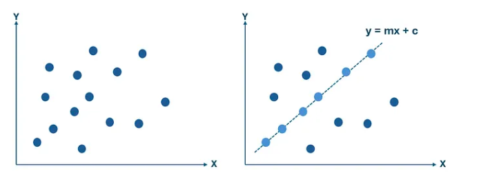
Slope-intercept form: y = mx + b
To detect lines mathematically, we begin with the standard slope-intercept equation. Here, m represents the slope of the line and b represents the intercept with the y-axis. Thus, detecting a line is equivalent to finding the correct pair (m, b) that best describes the observed edge points.
Standard line equation: y = m·x + b
m = slope (rise over run)
b = y-intercept
Goal: for a set of edge pixels, find the (m, b) pair
that most of them agree upon.
Image Space vs Parameter Space — The Key Insight
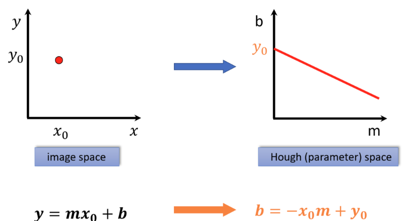
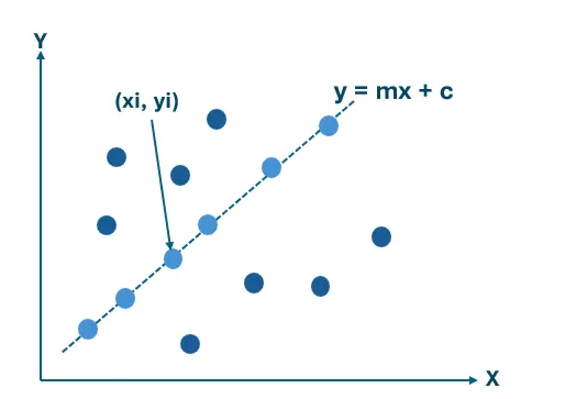
A point in image space becomes a line in parameter space
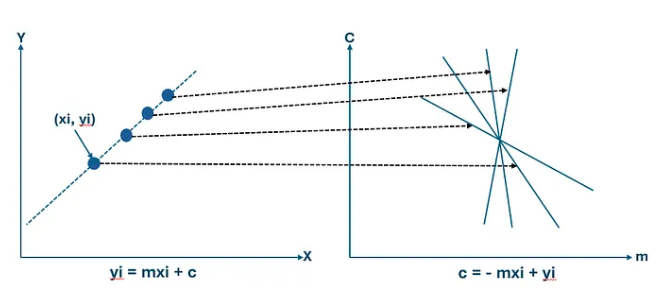
Each edge point (xᵢ, yᵢ) in the image contributes evidence about possible line parameters. Rearranging the line equation gives: b = −xᵢ·m + yᵢ. We observe that a single image point corresponds to a line in parameter space, and multiple image points belonging to the same physical line intersect at a common parameter pair (m, b). Therefore, intersections in parameter space indicate the presence of a line in image space.
Rearranging y = mx + b for a fixed image point (xᵢ, yᵢ):
b = −xᵢ · m + yᵢ
This is a LINE in (m, b) parameter space.
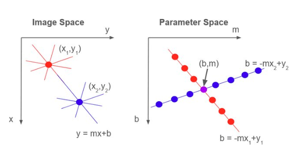
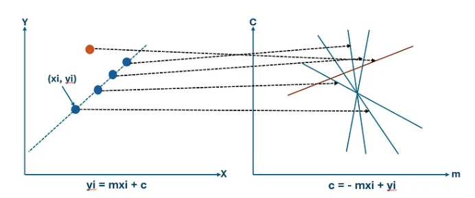
Key observations:
┌─────────────────────────────────────────────────────────┐
│ One image point → One line in parameter space │
│ N image points on same physical line → N lines in │
│ parameter space that all intersect at ONE point (m*,b*)│
│ That intersection = the detected line parameters │
└─────────────────────────────────────────────────────────┘
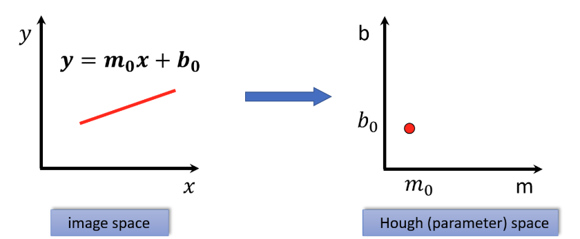
Line in image space ⟺ Point in parameter space
Image Space
Contains edge pixels at (x, y)
A LINE is what we want to find
Points that lie on a line → form the line
Searching here is expensive (all pairs)
Parameter Space (m, b)
Each image point → a line in this space
A LINE in image space → a POINT here
Intersection = line parameters
Searching here is efficient (voting)
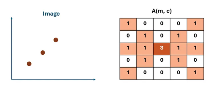
Voting Interpretation of the Hough Transform
The Hough Transform can be interpreted as a voting procedure. Each edge pixel votes for all parameter combinations that could represent a line passing through that pixel. These votes are accumulated inside a structure called the accumulator array. After processing all edge pixels, peaks in the accumulator correspond to detected lines. Higher peaks indicate stronger evidence for a line. A peak means many edge points agree on the same line parameters.
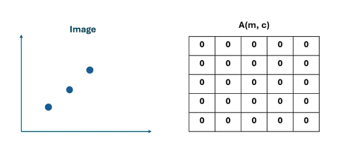
Accumulator Array (Discretized Parameter Space)
Parameter space divided into bins; each bin stores vote count
Instead of searching continuously over all parameter values, we discretize the parameter space into small regions called bins. Each bin stores the number of votes received from edge points. Each edge point contributes votes to the accumulator. The bin with the highest vote count represents the most likely line.
Accumulator array A(m, b):
Step 1: Quantize parameter space → finite grid of (m, b) bins
Step 2: Initialize A(m, b) = 0 for all bins
Step 3: For each edge point (xᵢ, yᵢ):
For each possible m value:
Compute b = yᵢ − m·xᵢ
Increment: A(m, b) = A(m, b) + 1
Step 4: Find peaks in A(m, b)
Step 5: Each peak (m*, b*) → detected line y = m*x + b*
Limitations of Slope-Intercept Representation
Why slope-intercept breaks down in practice
Although the slope-intercept representation y = mx + b is intuitive, it suffers from several practical limitations when used inside the Hough Transform framework. In particular: the slope parameter m can take values in the range −∞ to +∞, which makes parameter quantization difficult; representing nearly vertical lines becomes numerically unstable; and the accumulator array becomes unnecessarily large. To overcome these issues, we introduce a more stable representation called the polar representation of a line, which replaces slope and intercept with distance and angle parameters.
Problems with (m, b)
m ∈ (−∞, +∞) — unbounded range
Vertical lines: m → ∞ (undefined)
Accumulator must be very large
Quantization is non-uniform
Solution: Polar Form (ρ, θ)
θ ∈ [0°, 180°) — bounded, no duplicate endpoint
ρ bounded by image diagonal
Handles vertical lines perfectly
Compact, uniform accumulator
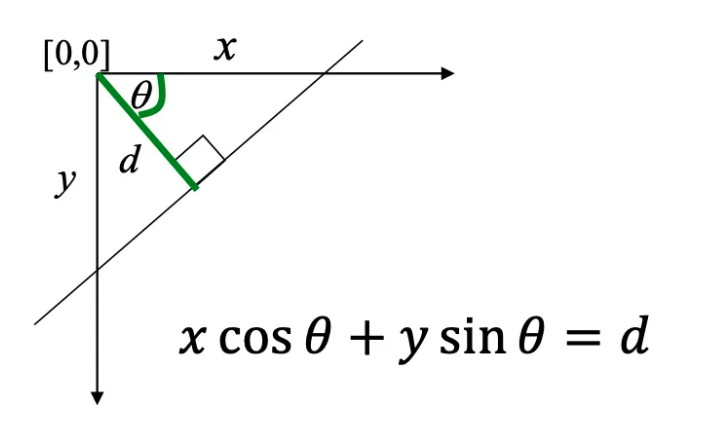
Polar Representation of a Line
Describe a line using distance ρ and angle θ instead of slope and intercept
Instead of describing a line using slope and intercept, we represent it using two parameters: θ is the angle between the perpendicular to the line and the x-axis, and ρ is the perpendicular distance from the origin to the line. The equation of the line becomes: x cos θ + y sin θ = ρ. This representation ensures that θ lies within a finite interval 0 ≤ θ ≤ π and ρ remains bounded by the image size. Therefore, the parameter space becomes compact and easier to discretize.
theta is the orientation of the unit normal n, not the direction along the line.
For an image of width W and height H with origin at a corner,
|rho| <= D = sqrt(W^2 + H^2). A common unique convention is theta in [0, pi)
with signed rho in [-D,D].
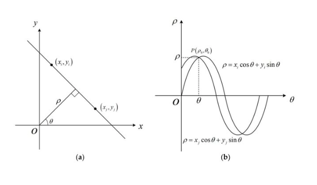
Why One Image Point Becomes a Sinusoidal Curve
In Hough space, one fixed image point traces a sinusoid as θ varies
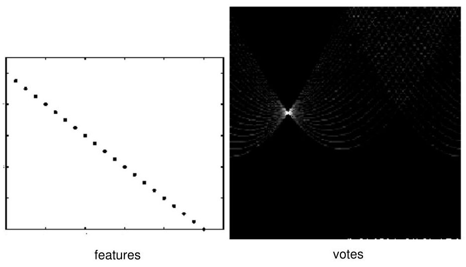
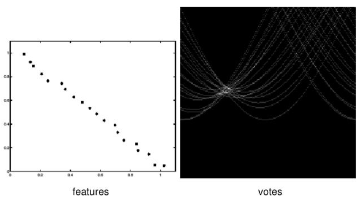
In the polar Hough Transform, a line is represented as ρ = x cos θ + y sin θ. Now assume we have one fixed edge point (xᵢ, yᵢ) in the image. For this point, there are many possible lines that can pass through it — each possible line has a different angle θ. For every chosen value of θ, we compute a corresponding value of ρ = xᵢ cos θ + yᵢ sin θ. Therefore, the same image point produces many possible parameter pairs (ρ, θ). When these pairs are plotted in Hough space, they form a sinusoidal curve. The sinusoidal shape arises directly from the form of the polar line equation.
For a fixed image point \((x_i,y_i)\),
\[
\rho_i(\theta)=x_i\cos\theta+y_i\sin\theta.
\]
As \(\theta\) varies, this traces a sinusoid in \((\rho,\theta)\) space. Every point on the curve represents one candidate line through \((x_i,y_i)\).
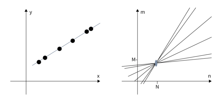
How Multiple Points Reveal a Line
Sinusoidal curves from collinear points intersect at a common (ρ*, θ*)
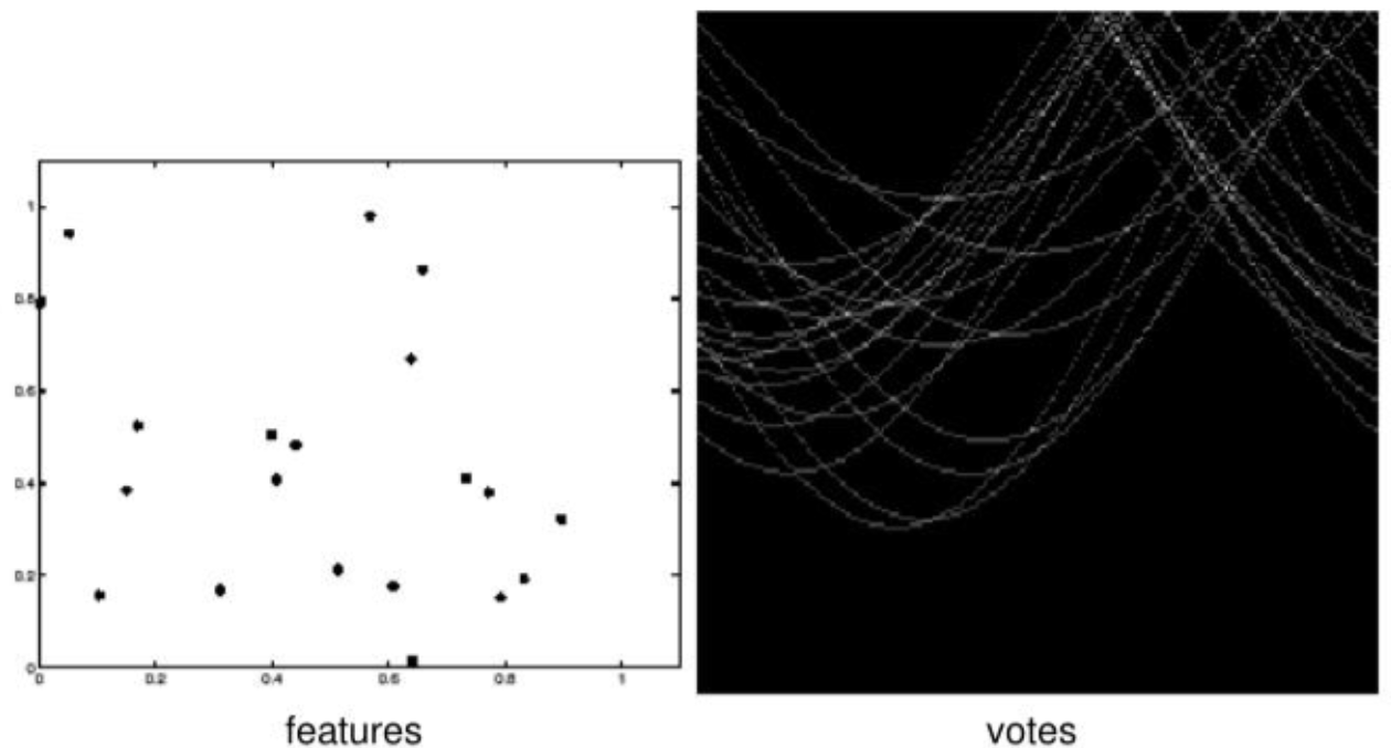
If several edge points lie on the same physical line in the image, then they all share one common line parameter pair (ρ*, θ*). This means each edge point produces its own sinusoidal curve in Hough space, and the curves from points on the same line intersect at the same location. This intersection receives many votes in the accumulator array. Therefore, a strong peak in Hough space indicates a detected line in the image.
N collinear image points → N sinusoidal curves in Hough space
All N curves pass through the same point (ρ*, θ*)
This point receives N votes from the accumulator.
The more points on the line → the higher the peak.
┌───────────────────────────────────────────┐
│ Line in image space ⟺ Peak in Hough space│
└───────────────────────────────────────────┘
The Core Duality
Image space and Hough (parameter) space are dual to each other. A point in image space becomes a sinusoidal curve in Hough space. A line in image space becomes a peak in Hough space. Detection in Hough space is equivalent to finding where many curves intersect — which is exactly what the voting accumulator computes.
Discretizing the Accumulator Space
The parameter space is continuous, so we cannot store every possible value of ρ and θ directly. Instead, we divide the parameter space into small bins. Δρ controls the distance resolution. Δθ controls the angle resolution. Each computed parameter pair (ρ, θ) is mapped to an accumulator bin. The bin indices are computed as: ρᵢ = round(ρ / Δρ) and θⱼ = round(θ / Δθ). Then the corresponding accumulator cell is incremented: H(ρᵢ, θⱼ) = H(ρᵢ, θⱼ) + 1.
With lower bounds \(\rho_{\min}\) and \(\theta_{\min}\), robust bin indices are
\[
i=\operatorname{round}\!\left(\frac{\rho-\rho_{\min}}{\Delta\rho}\right),\qquad
j=\operatorname{round}\!\left(\frac{\theta-\theta_{\min}}{\Delta\theta}\right),
\qquad H[i,j]\leftarrow H[i,j]+w.
\]
Standard voting uses \(w=1\); weighted Hough voting may use edge magnitude or another confidence. Large bins merge nearby lines; very fine bins scatter votes under noise and quantization.
Bins Too Large
Different lines merge into single peak
Cannot distinguish closely spaced lines
Detection accuracy reduced
Bins Too Small
Votes scatter over many bins
True peaks become hard to find
Noise creates false peaks
Why Use a Half-Open 180° Angle Range?
The pairs \((\rho,\theta)\) and \((-\rho,\theta+\pi)\) describe the same geometric line. A half-open interval of length \(\pi\), such as \([0,\pi)\) or \([-\pi/2,\pi/2)\), removes this redundancy when \(\rho\) is signed. The half-open endpoint matters: including both endpoints duplicates one orientation.
Edge detection: Run Canny, Sobel, or another edge detector on the input image to produce an edge map.
2
Initialize accumulator: Create a 2D accumulator array H(ρ, θ) = 0. Dimensions are determined by the chosen Δρ and Δθ resolution.
3
Vote for each edge pixel: For each detected edge point (x, y), iterate over all candidate angles −90° ≤ θ ≤ 90°. For each θ, compute ρ = x cos θ + y sin θ. Increment the accumulator cell H(ρ, θ) = H(ρ, θ) + 1.
4
Find peaks: Locate local maxima in the accumulator array. A peak means many edge pixels voted for the same (ρ, θ) — indicating a strong line candidate.
5
Threshold and filter: Keep only peaks above a vote-count threshold. Apply non-maximum suppression to remove nearby weaker peaks.
6
Convert to lines: Each remaining peak (ρ*, θ*) corresponds to the detected line: x cos θ* + y sin θ* = ρ*. Draw or output these lines on the original image.
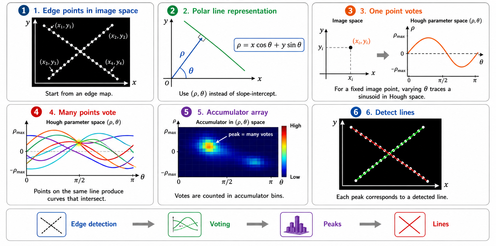
6-Step Line Detection Flow
Edge PointsStart from edge map
→
Polar Formρ = x cosθ + y sinθ
→
One Point VotesSinusoid in Hough space
→
Many Points VoteCurves intersect
→
AccumulatorPeaks = votes
→
Detect LinesPeak → line params
From Accumulator Peaks to Final Lines
After the accumulator array is filled, we do not directly accept every peak as a detected line. Instead, we apply filtering steps. First, threshold the accumulator: keep only bins whose vote count is high enough. Second, apply non-maximum suppression: keep only local maxima and remove nearby weaker peaks. Third, extract the corresponding lines: convert each remaining peak (ρ, θ) back into a line in the image. The final output is a set of reliable detected lines rather than all possible accumulator responses.
Post-processing:
1. Thresholding:
Accept peak at (ρᵢ, θⱼ) only if H(ρᵢ, θⱼ) ≥ T_min
2. Non-maximum suppression:
For each candidate peak, check if it is a local maximum
in its neighborhood. Keep only local maxima.
3. Line extraction:
Convert each (ρ*, θ*) → line equation:
x·cos θ* + y·sin θ* = ρ*
This line is projected back onto the image.
Result: A clean set of detected lines from noisy edge data.
Gradient-Guided Hough Voting — Faster and More Accurate
Use gradient orientation to reduce voting to a single θ per pixel
In the standard Hough Transform, each edge pixel votes for many possible values of θ. This is computationally expensive and may also create unnecessary votes in the accumulator. A better idea is to use the gradient orientation already computed during edge detection. The gradient direction θg = atan2(∂f/∂y, ∂f/∂x) points in the direction of the strongest intensity change — perpendicular to the local edge boundary. In the polar line equation, the angle θ represents the direction of the normal to the line. Therefore, the gradient orientation can be used as a direct estimate for θ, or voting can be restricted to a small interval around it. This reduces computation because each edge pixel votes for fewer possible lines.
Standard Hough: each edge pixel votes for ALL θ values in [−90°, 90°]
→ O(N_edge × N_θ) votes total
Gradient-Guided Hough:
1. Detect edge pixels with Sobel/Canny
2. For each edge pixel (x, y), compute:
θg = atan2(∂f/∂y, ∂f/∂x) ← gradient direction ⊥ to edge
3. Vote ONLY for θ ≈ θg (or a narrow range around θg)
4. Compute: ρ = x·cos θg + y·sin θg
5. Increment: H(ρ, θg) = H(ρ, θg) + 1
→ Approximately O(N_edge) votes when one angle is used per pixel
→ Fewer false accumulator peaks
→ Faster computation
Why Gradient Direction ≈ θ in Polar Form
In the polar line equation ρ = x cos θ + y sin θ, the angle θ is the orientation of the line's normal vector — pointing perpendicular to the line. The image gradient ∇f also points perpendicular to the edge boundary. Therefore, the gradient direction at an edge pixel is a direct estimate of the line normal θ in the Hough polar representation. Using this allows each pixel to vote for just one θ value instead of all possible angles.
Choosing Accumulator Cell Size
The accuracy of the Hough Transform depends strongly on the choice of accumulator resolution. If accumulator bins are too large, different lines may merge into a single peak. If accumulator bins are too small, votes become scattered and true peaks become harder to detect. Therefore, selecting an appropriate discretization of parameter space is essential for reliable detection.
Detecting Multiple Lines
After constructing the accumulator array, line detection is performed by locating local maxima in parameter space. However, noisy edge points may generate false peaks, weak edges may generate low peaks, and overlapping structures may produce multiple candidate peaks. Thus, additional constraints such as thresholding and non-maximum suppression are often required to improve robustness. Multiple lines can be detected simultaneously by finding multiple peaks — each peak independently corresponds to one detected line.
Circle Representation in the Hough Transform
A circle described by center (a, b) and radius r
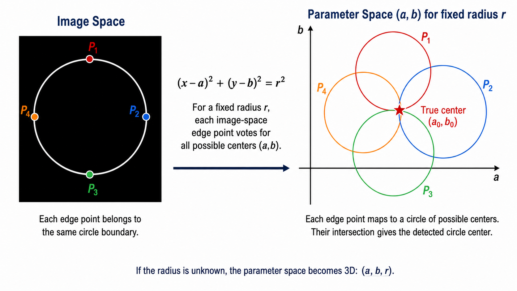
A circle can be represented by the equation: (x − a)² + (y − b)² = r², where (x, y) is an edge pixel lying on the circle boundary, (a, b) is the circle center, and r is the circle radius. For circle detection, the parameter space becomes (a, b, r) — three-dimensional if the radius is unknown, or two-dimensional if the radius is fixed.
\[
(x-a)^2+(y-b)^2=r^2
\]
Known r: parameter space is 2D (a,b); each boundary point votes for a circle of
possible centers. Unknown r: parameter space is 3D (a,b,r); each point contributes a
conical surface. Peaks estimate (a0,b0) or (a0,b0,r0), respectively.
Image Space to 2D Parameter Space (Known Radius)
Each edge point maps to a circle of possible centers
When the radius r is known, each edge point (x, y) on the circle boundary constrains the center (a, b) to lie on a circle of radius r centered at (x, y). Multiple edge points belonging to the same circle will map to circles in parameter space that all intersect at the true center (a₀, b₀). This intersection receives many votes and corresponds to the detected circle center. With just three or more non-collinear edge points, the center can be precisely located.
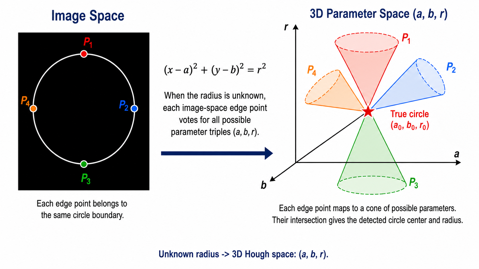
Image Space to 3D Parameter Space (Unknown Radius)
Unknown radius → each point votes for a cone in (a, b, r) space
When the radius is unknown, each image-space edge point votes for all possible parameter triples (a, b, r). In 3D parameter space, this creates a cone of possible parameters. The intersection of cones from multiple edge points gives the detected circle center and radius simultaneously. The accumulator becomes 3D — much larger than the 2D case. Gradient information is therefore especially important to reduce computation in 3D.
Why Gradient Information Helps in Circle Detection
The gradient direction points approximately along the radius direction
Gradient information is very useful in circle detection because the geometry of a circle gives an important constraint. At a circle boundary, the edge direction is tangent to the circle. The gradient direction is perpendicular to the edge boundary. Therefore, the gradient direction points approximately along the radius direction — connecting the boundary point to the center. Since the radius connects the boundary point to the center, the circle center must lie approximately along the gradient direction or the opposite gradient direction. This means that the edge pixel does not need to vote for all possible centers.
For an edge pixel \((x,y)\), gradient angle \(\theta_g\), and candidate radius \(r\):
\[
(a,b)=\bigl(x\pm r\cos\theta_g,\ y\pm r\sin\theta_g\bigr).
\]
The two signs account for unknown edge polarity. If polarity is known, one direction may suffice. If \(r\) is unknown, repeat over candidate radii; gradient guidance reduces center votes but does not remove the radius dimension.
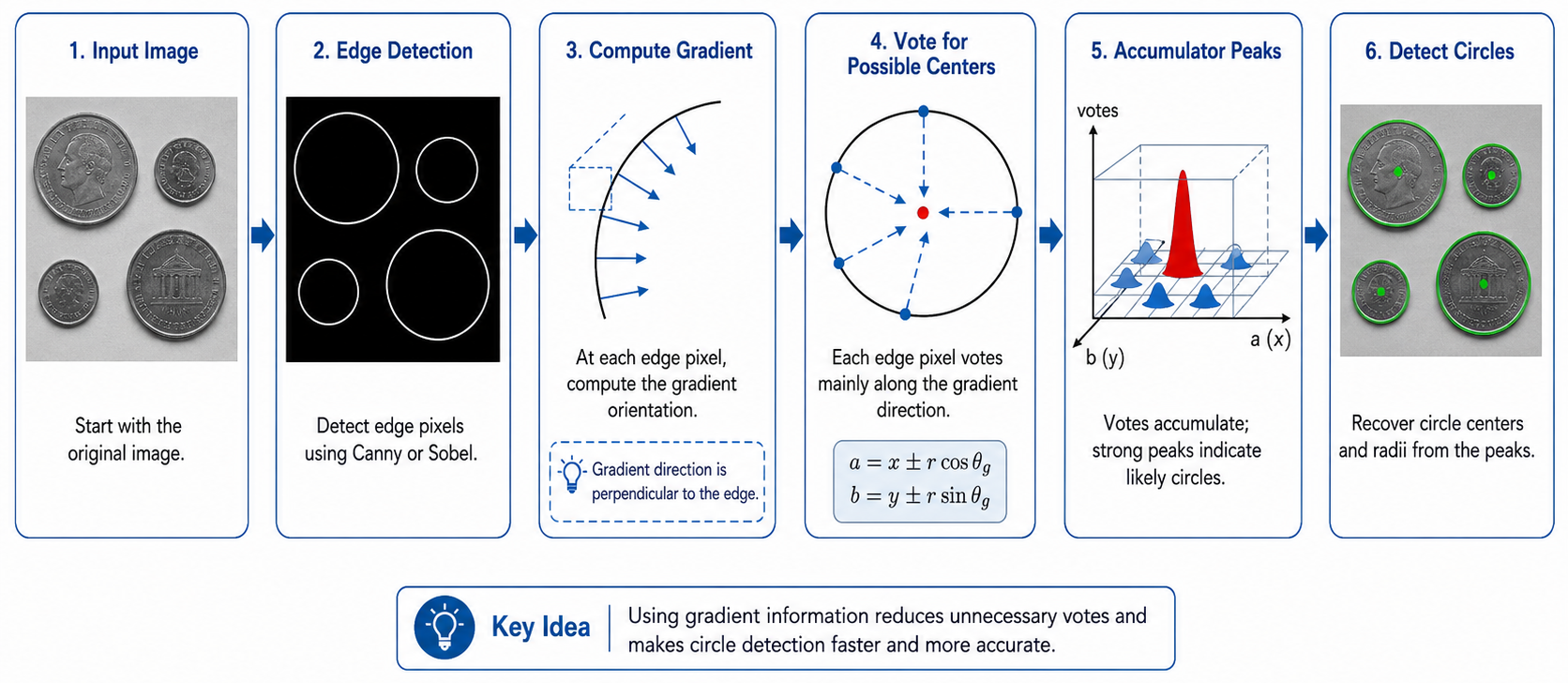
Gradient-Guided Circle Detection Pipeline
1
Input image: Start with the original image.
2
Edge detection: Detect edge pixels using Canny or Sobel to find circle boundary pixels.
3
Compute gradient: At each edge pixel, compute the gradient orientation θg = atan2(∂f/∂y, ∂f/∂x). The gradient direction is perpendicular to the edge — and therefore points along the radius toward the circle center.
4
Vote for possible centers: Each edge pixel votes mainly along the gradient direction: a = x ± r cos θg, b = y ± r sin θg. This dramatically reduces the number of votes compared to voting for all possible centers.
5
Accumulator peaks: Votes accumulate in the (a, b) accumulator. Strong peaks indicate likely circle centers. A peak at (a₀, b₀) means many edge pixels' gradients converge there.
6
Detect circles: Recover circle centers and radii from the accumulator peaks. Each peak (a₀, b₀) with the known radius r gives a fully specified detected circle.
Extensions of the Hough Transform
The Hough Transform provides a flexible framework for detecting geometric structures in images. It can be extended to detect: ellipses, using center, axes, and orientation parameters; rectangles, using line combinations and geometric constraints; and arbitrary parametric shapes, when the shape can be described mathematically. Additionally, stronger edges can be assigned larger vote weights, gradient information can restrict the voting direction, and parameter sampling resolution can be adjusted to balance accuracy and speed.
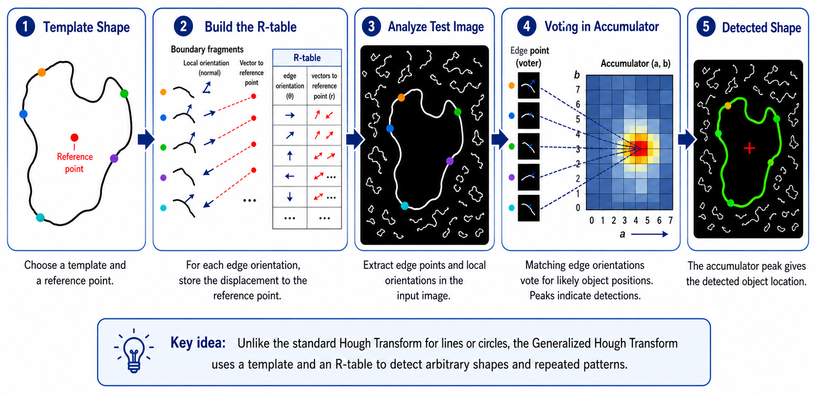
Generalized Hough Transform for Irregular Shape Detection
Detect arbitrary shapes using a template and an R-table
Unlike the standard Hough Transform for lines or circles, the Generalized Hough Transform uses a template and an R-table to detect arbitrary shapes and repeated patterns. The idea is to encode the shape's boundary structure into a lookup table indexed by local gradient orientation.
1
Template shape: Choose a template object and designate a reference point (e.g., the centroid).
2
Build the R-table: For each boundary pixel of the template, record its gradient orientation θ and the displacement vector r from that pixel to the reference point. Group entries by orientation θ. The R-table maps: edge orientation θ → list of displacement vectors to reference point.
3
Analyze test image: Detect edge points and compute their local gradient orientations in the input image.
4
Voting in accumulator: For each test edge pixel with orientation θ, look up the R-table entry for θ. For each displacement vector r stored there, vote for the position (x + r.x, y + r.y) as a possible reference point location in the accumulator.
5
Detected shape: The accumulator peak gives the detected object location. The location of the peak corresponds to where the reference point of the template is located in the test image.
Generalized Hough — Key Idea
The R-table encodes the relationship between local edge orientations and the object's reference point. During detection, matching edge orientations in the test image vote for likely object positions using stored displacement vectors. This allows recognition of any shape — not just analytically defined ones like lines or circles.
Summary Comparison
Shape
Parameters
Param Space Dim
Each Point Votes For
Notes
Line (slope-intercept)
m, b
2D
A line in (m,b) space
Unbounded; problematic for vertical lines
Line (polar)
ρ, θ
2D
A sinusoidal curve in (ρ,θ)
Bounded; handles all orientations
Circle (known r)
a, b
2D
A circle of centers in (a,b)
Gradient reduces to 2 votes
Circle (unknown r)
a, b, r
3D
A cone in (a,b,r)
Computationally expensive
Arbitrary (GHT)
Reference point
2D+
Displacement via R-table
Requires template; handles any shape
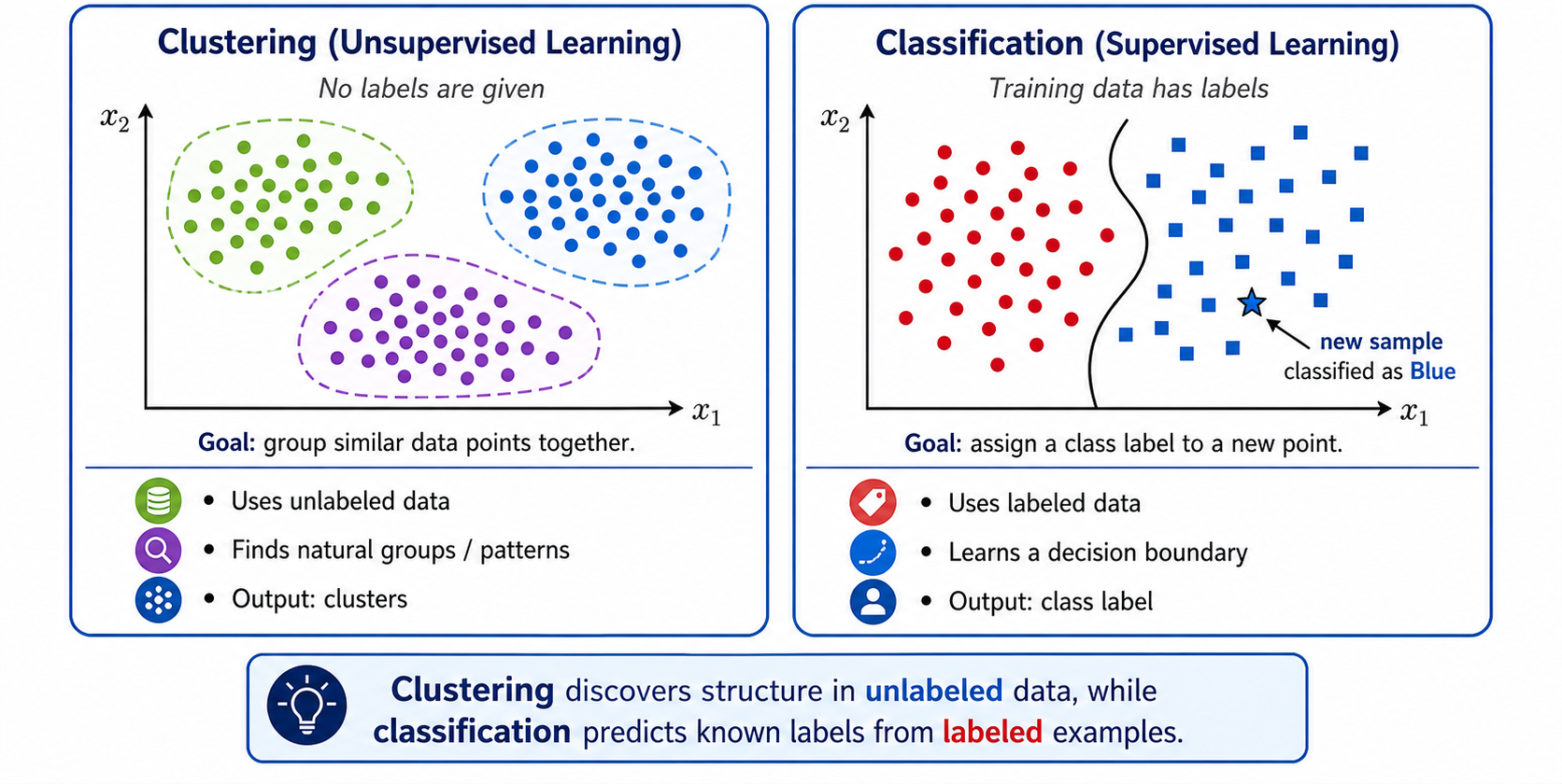
Clustering vs Classification
Clustering — Unsupervised
No class labels are supplied
Discovers groups by feature similarity
Output: cluster assignments and centers
Example: K-means segmentation
Classification — Supervised
Learns from labeled examples
Predicts predefined class labels
Separate training and prediction phases
Examples: SVM, KNN, trees
Important: K-means cluster IDs are arbitrary, not semantic labels. “Cluster 1” does not automatically mean “car” or “sky.” Classification learns semantic labels from labeled training data.
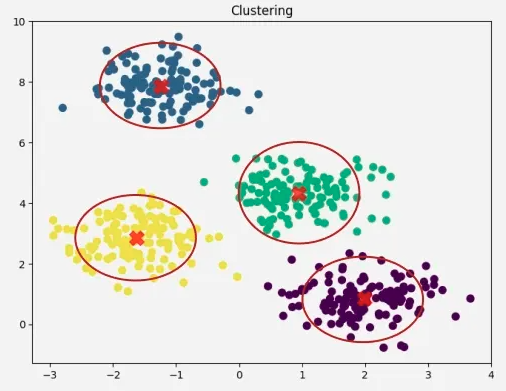
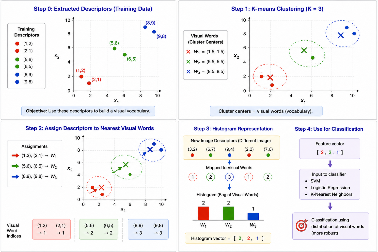
K-Means Objective
Partition points into K compact clusters
Given feature vectors \(\{\mathbf{x}_n\}_{n=1}^{N}\), K-means minimizes the within-cluster sum of squared Euclidean distances. The assignments and centroids are coupled, so the algorithm alternates between optimizing one while holding the other fixed.
Assignment chooses the nearest centroid. Update replaces each centroid by the mean of
its assigned points. Each non-degenerate step does not increase J, but convergence is only
to a local optimum and depends on initialization.
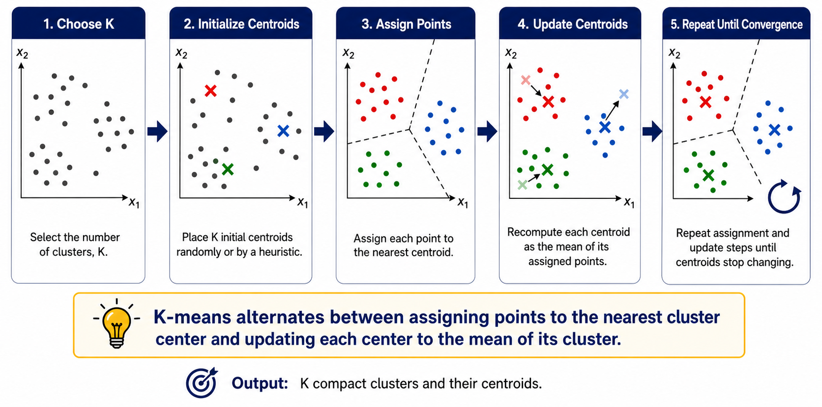
Complete K-Means Algorithm
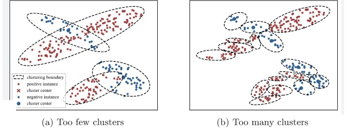
1
Choose K. Too small can merge distinct regions (under-segmentation); too large can split meaningful regions (over-segmentation).
2
Initialize K centroids. Random initialization is sensitive; k-means++ is a common improvement. Multiple restarts help find a lower objective.
3
Assign every point to its nearest centroid using the chosen distance and consistently scaled features.
4
Update every nonempty centroid to the arithmetic mean of its assigned points; handle empty clusters explicitly.
5
Repeat until assignments or centroids stabilize, improvement in \(J\) is below tolerance, or the iteration limit is reached.
Lecture Numerical Example — K = 2
Data: \((185,72),(170,56),(168,60),(179,68),(182,72),(188,77)\). Initial centroids are \(\mu_1=(185,72)\), \(\mu_2=(170,56)\). Nearest-centroid assignment gives \(C_1=\{(185,72),(179,68),(182,72),(188,77)\}\) and \(C_2=\{(170,56),(168,60)\}\).
Correction to the original text: the second updated centroid is (169,58), not
(169.5,58). The assignments remain unchanged after this update, so the example converges.
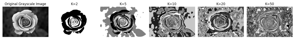
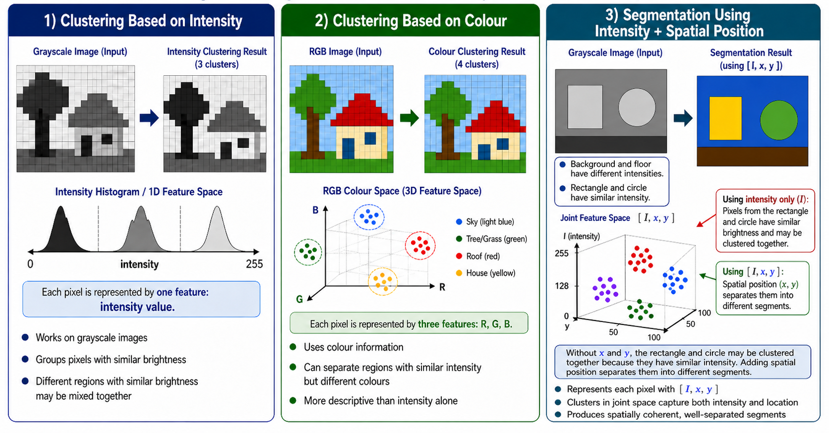
K-Means for Image Segmentation
Pixel feature
Dimension
What it groups
Main caution
\([I]\)
1
Similar brightness
Distant objects with similar intensity may merge
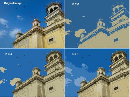
\([R,G,B]\)
3
Similar colors
Ignores spatial coherence
\([I,x,y]\)
3
Brightness and proximity
Feature scales must be balanced
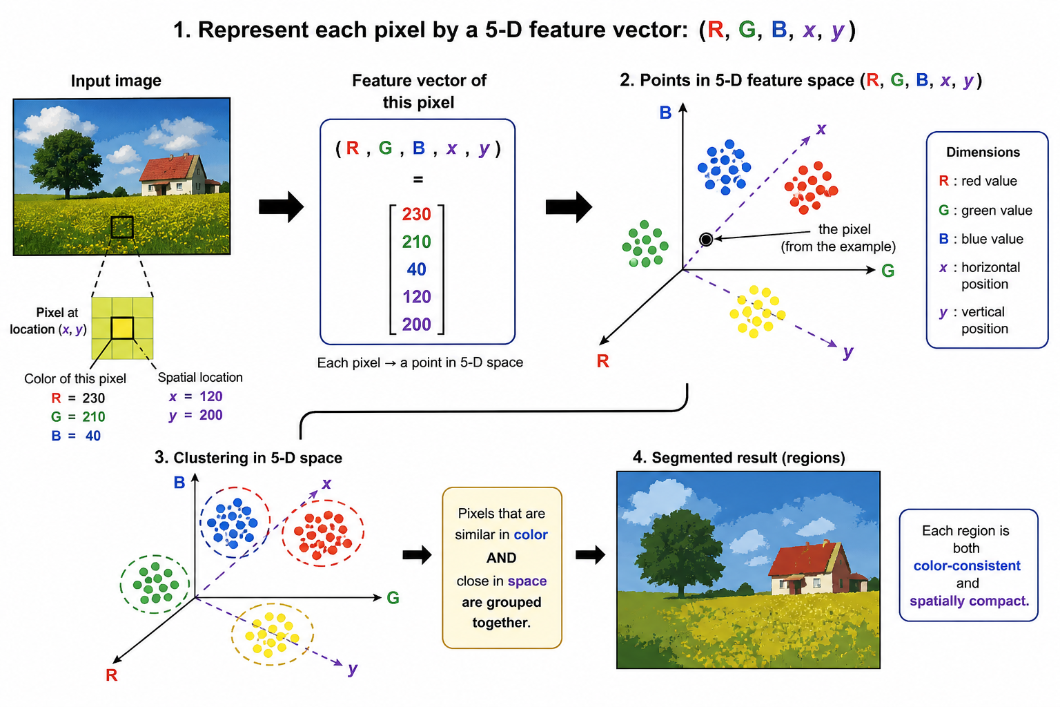
\([R,G,B,x,y]\)
5
Color-consistent, compact regions
Raw coordinates can dominate without scaling
A useful weighted feature is
\[
\mathbf{z}(x,y)=\left[R,G,B,\lambda_x x,\lambda_y y\right]^T,
\]
where the \(\lambda\) values control the trade-off between appearance similarity and spatial compactness.
Advantages
Simple and usually fast
Scales to many points
Centroids are intuitive prototypes
Useful for segmentation and codebooks
Limitations
K must be selected
Sensitive to initialization and outliers
Local, not guaranteed global, optimum
Favors compact convex/spherical clusters
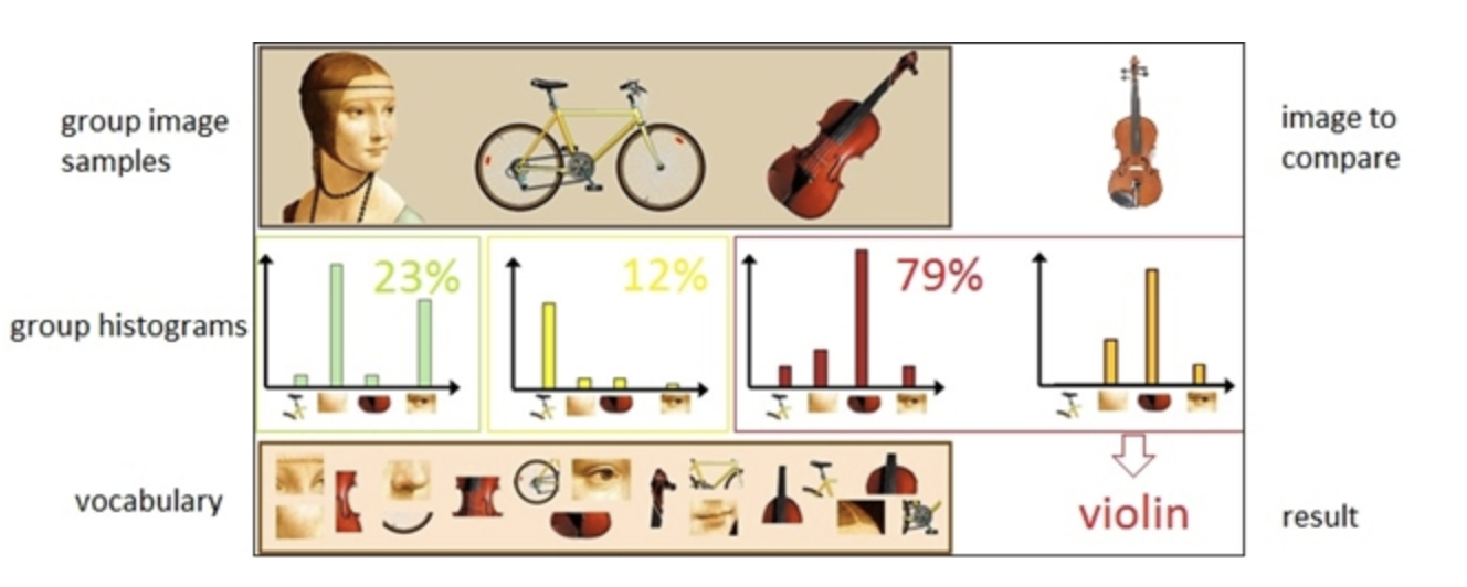
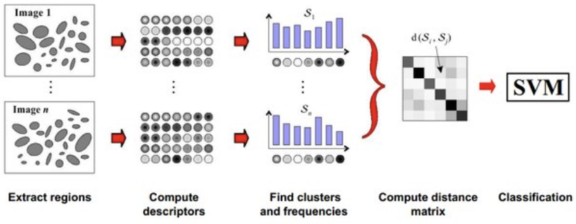
Why Bag of Visual Words?
Variable local descriptors become one fixed-length image vector
Different images contain different numbers of keypoints. BoVW quantizes their local descriptors against a vocabulary learned from training descriptors only, then counts visual-word occurrences. A vocabulary of size \(K\) produces a \(K\)-dimensional histogram for every image.
Detectinterest points
→
DescribeSIFT/other local descriptor
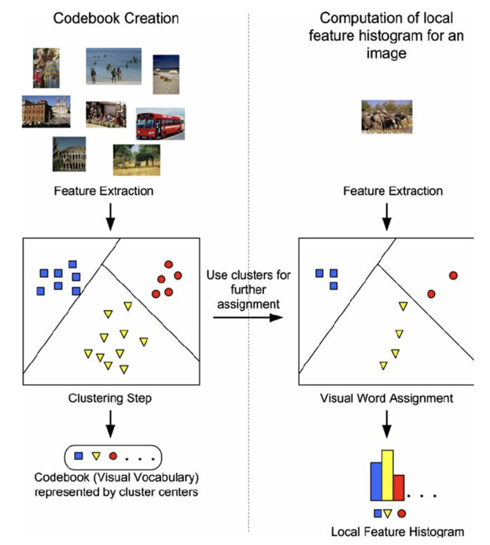
→
Cluster Training DescriptorsK-means codebook
→
Quantizenearest visual word
→
Histogramfixed K dimensions
→
Classifyfor example, SVM
Vocabulary, Quantization, and Histogram
Let the learned visual words be \(\{\mathbf{w}_k\}_{k=1}^{K}\). For descriptor \(\mathbf{d}_j\):
\[
q(\mathbf{d}_j)=\arg\min_{k\in\{1,\ldots,K\}}
\lVert\mathbf{d}_j-\mathbf{w}_k\rVert_2^2,
\qquad
h_k=\sum_{j=1}^{M}\mathbf{1}\!\left[q(\mathbf{d}_j)=k\right]
\]
Each centroid w_k is a visual word. Hard assignment maps each descriptor to one word.
The histogram discards exact descriptor order and much spatial layout; this is both a source
of robustness and a limitation. Spatial pyramids can restore coarse layout information.
Histogram Normalization and Similarity
\[
\mathbf{h}_{L1}=\frac{\mathbf{h}}{\sum_k|h_k|},\qquad
\mathbf{h}_{L2}=\frac{\mathbf{h}}{\sqrt{\sum_kh_k^2}}
\]
\[
\operatorname{HI}(\mathbf{h},\mathbf{g})=\sum_k\min(h_k,g_k),\quad
\operatorname{cos}(\mathbf{h},\mathbf{g})=
\frac{\mathbf{h}^T\mathbf{g}}{\lVert\mathbf{h}\rVert_2\lVert\mathbf{g}\rVert_2},\quad
d_2(\mathbf{h},\mathbf{g})=\lVert\mathbf{h}-\mathbf{g}\rVert_2
\]
Normalization prevents images with more detected keypoints from dominating merely because their raw counts are larger.
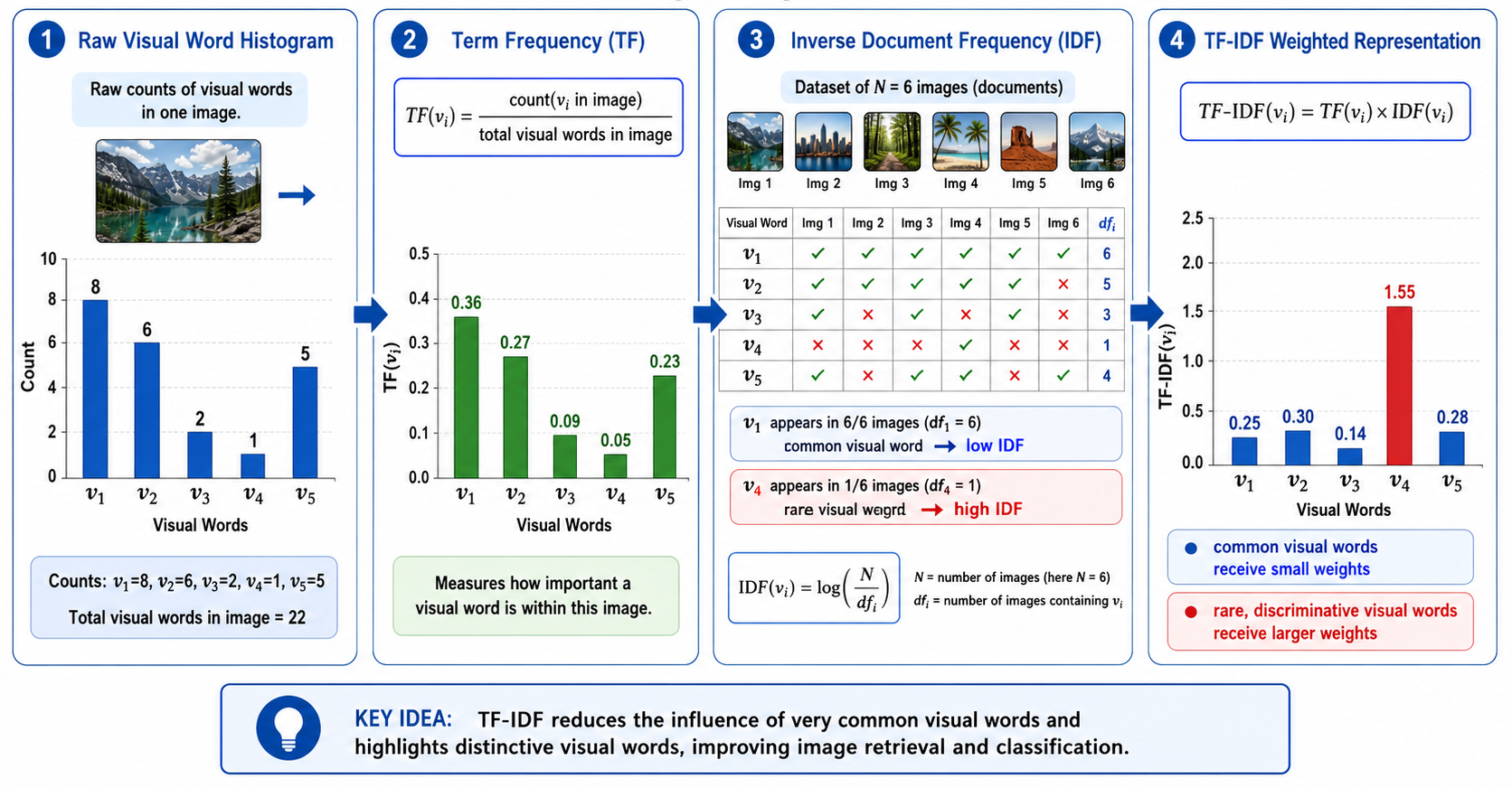
TF-IDF Weighting
For image \(d\), vocabulary word \(k\), and \(N\) training images:
\[
\operatorname{tf}_{k,d}=\frac{n_{k,d}}{\sum_jn_{j,d}},\qquad
\operatorname{idf}_k=\log\!\left(\frac{N}{\operatorname{df}_k}\right),\qquad
t_{k,d}=\operatorname{tf}_{k,d}\operatorname{idf}_k
\]
Common words have large document frequency and low IDF; rare words receive more weight. In software, a smoothed IDF such as \(\log((N+1)/(\mathrm{df}_k+1))+1\) avoids zero or undefined edge cases.
Lecture TF-IDF example — corrected arithmetic
For counts \([8,6,2,1,5]\), total 22, \(N=6\), and document frequencies \([6,5,3,1,4]\), natural-log TF-IDF is approximately \([0,0.0497,0.0630,0.0814,0.0921]\). The original listed values \([0.25,0.30,0.14,1.55,0.28]\) do not follow its stated formulas. Different log bases or smoothing change scale, but the formula must be applied consistently.
BoVW Numerical Example — Correct Nearest-Word Assignment
Vocabulary: \(W_1=(1.5,1.5)\), \(W_2=(5.5,5.5)\), \(W_3=(8.5,8.5)\). New descriptors: \((3,2),(6,7),(9,4),(2,2),(7,6)\). The original lecture assigns \((9,4)\) to \(W_3\), but the distances show it belongs to \(W_2\).
\[
\lVert(9,4)-W_1\rVert_2=\sqrt{62.5},\quad
\lVert(9,4)-W_2\rVert_2=\sqrt{14.5},\quad
\lVert(9,4)-W_3\rVert_2=\sqrt{20.5}
\]
Therefore \((9,4)\to W_2\). All assignments are
\[
(3,2)\to W_1,\ (2,2)\to W_1,\
(6,7)\to W_2,\ (9,4)\to W_2,\ (7,6)\to W_2,
\]
so the correct raw histogram is \(\boxed{[2,3,0]}\), not \([2,2,1]\).
BoVW robustness to rotation or scale is not automatic; it depends heavily on the detector/descriptor (for example, SIFT) and the pooling design. BoVW is naturally insensitive to permutation of local descriptors and moderately tolerant of small spatial rearrangements.
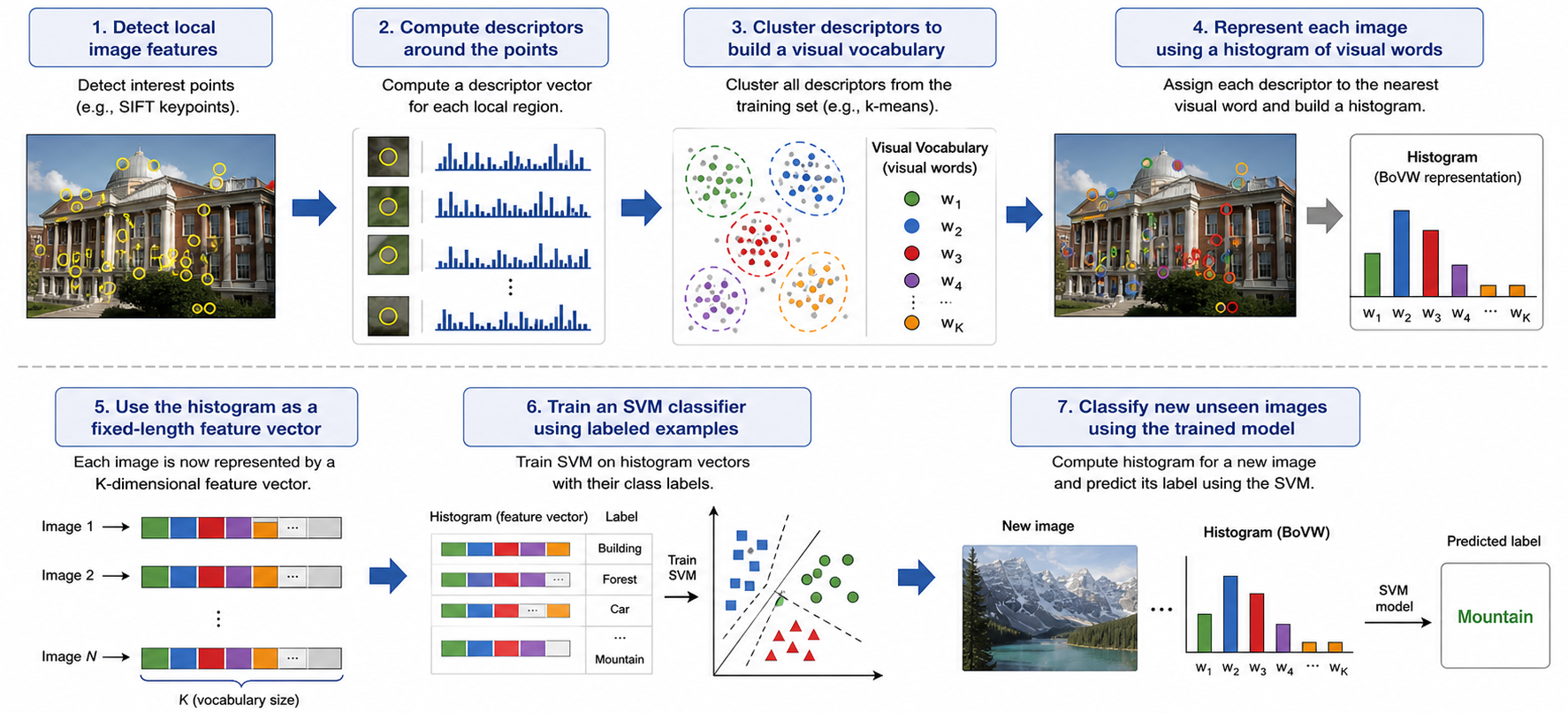
Why SVM After BoVW?
BoVW represents; SVM decides
BoVW converts each image into a fixed-length vector \(\mathbf{x}\in\mathbb{R}^{K}\). With labels \(y_i\in\{-1,+1\}\), an SVM learns a separating hyperplane. At prediction time, the vocabulary and classifier remain fixed: the new image is encoded with the training vocabulary and passed to the trained SVM.
Linear Decision Function and Geometry
\[
f(\mathbf{x})=\mathbf{w}^T\mathbf{x}+b,\qquad
\widehat{y}=\operatorname{sign}(f(\mathbf{x}))
\]
\[
\text{hyperplane: }\mathbf{w}^T\mathbf{x}+b=0,\qquad
\text{distance from }\mathbf{x}\text{ to it}=
\frac{|\mathbf{w}^T\mathbf{x}+b|}{\lVert\mathbf{w}\rVert_2}
\]
In the canonical scaling, the support planes are \(\mathbf{w}^T\mathbf{x}+b=\pm1\). Each side of the margin is \(1/\lVert\mathbf{w}\rVert_2\), so the full margin width is \(2/\lVert\mathbf{w}\rVert_2\).
C trades margin size against training violations: larger C penalizes violations more;
smaller C allows a wider, more regularized margin. Support vectors have active constraints
and determine the boundary; they are not simply every correctly classified point.
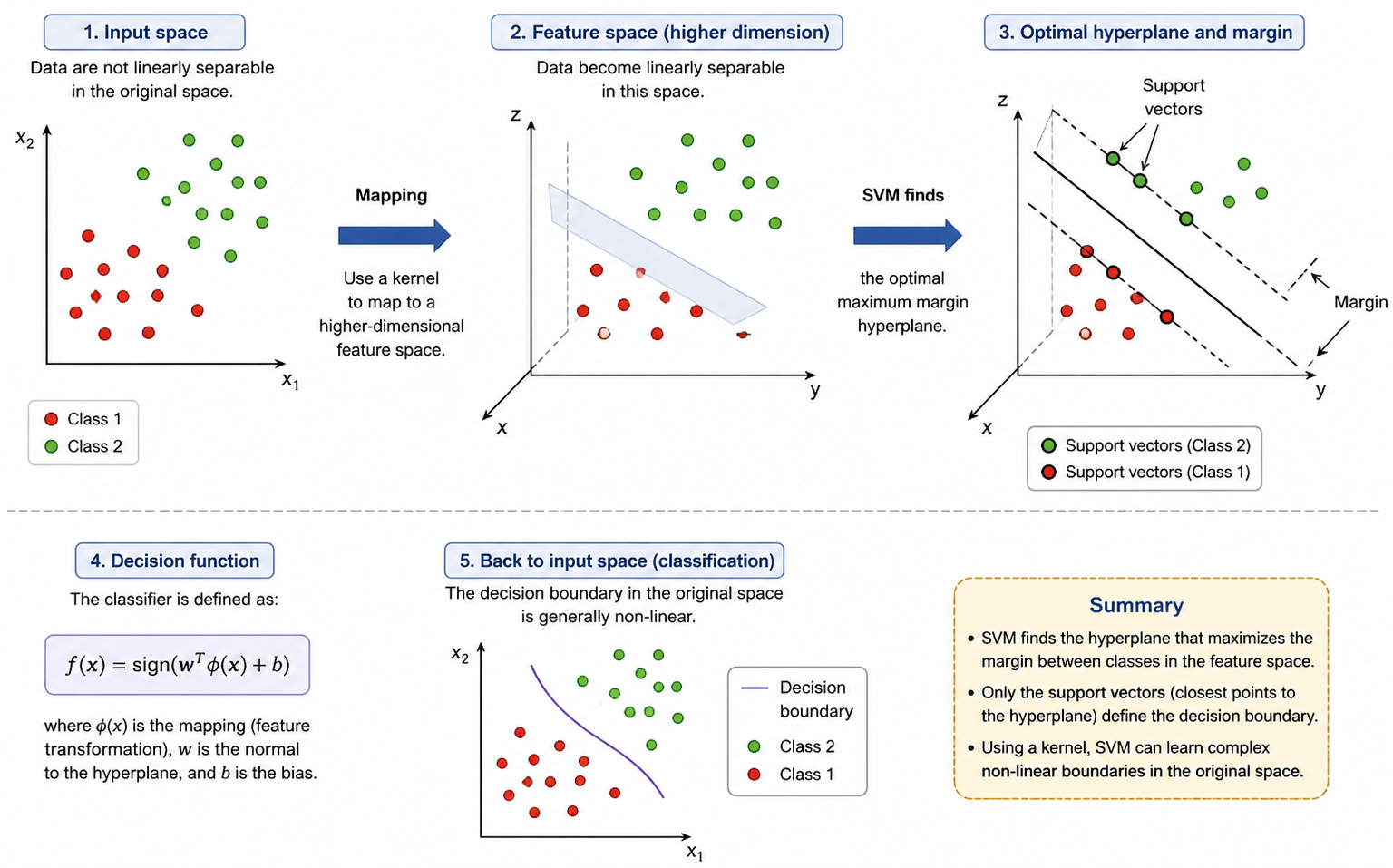
Nonlinear SVM and the Kernel Trick
A feature map \(\phi(\mathbf{x})\) can make data linearly separable in another space. A kernel evaluates inner products there without explicitly constructing all mapped coordinates: \(K(\mathbf{x},\mathbf{z})=\phi(\mathbf{x})^T\phi(\mathbf{z})\).
\[
\widehat{y}=\operatorname{sign}\!\left(
\sum_{i\in SV}\alpha_i y_iK(\mathbf{x}_i,\mathbf{x})+b\right)
\]
Common kernels include
\[
K_{\mathrm{linear}}(\mathbf{x},\mathbf{z})=\mathbf{x}^T\mathbf{z},\qquad
K_{\mathrm{RBF}}(\mathbf{x},\mathbf{z})=
\exp\!\left(-\gamma\lVert\mathbf{x}-\mathbf{z}\rVert_2^2\right).
\]
Training vs Prediction — Avoiding Data Leakage
Training phase
Prediction phase
Detect and describe training images
Detect and describe the unseen image
Fit K-means vocabulary on training descriptors
Assign descriptors to the existing vocabulary
Fit normalization/IDF using training data
Apply the same stored transformation
Train SVM on labeled histogram vectors
Predict with the fixed trained SVM
The vocabulary, IDF weights, normalization choices, and SVM hyperparameters must be learned or selected without using the test set. Fitting the codebook on test descriptors leaks information and makes evaluation optimistic.
Complete Classical Recognition Pipeline
Image
→
Keypoints
→
Descriptors
→
Visual Words
→
Normalized / TF-IDF Histogram
→
SVM Label
One-line memory aid
K-means discovers prototypes, BoVW turns a variable set of descriptors into a fixed histogram, and SVM learns the labeled decision boundary.
Hough Transform — Interactive Line Voting Simulator
Click on the image canvas to place edge points. Watch the Hough accumulator update in real time. Each point traces a sinusoidal curve. Where curves intersect, votes accumulate — revealing detected lines.
Image Space — click to add edge points
Hough Accumulator H(ρ, θ)
Points placed: 0
Sinusoidal Curve Explorer
Adjust x and y to see how an image point's sinusoidal curve changes in Hough space. The curve represents ρ(θ) = x·cosθ + y·sinθ.
Image point x100
Image point y80
Hough space: ρ(θ) = x·cosθ + y·sinθ
Polar Line Equation Calculator
θ (degrees)45°
ρ (pixels)50
Visual Cheat Sheet Summary
50-Question Practice Quiz
This comprehensive practice quiz contains 50 multiple-choice questions loaded directly from the lecture database.
Score: 0 / 0 answered
25-Question True/False Practice
Answer each statement, reveal optional hints, and review the explanation after submitting.
Figures Extracted from the Original Lecture Document
These figures are preserved in their original document order as a complete visual reference. Captions identify the source part and figure number; explanatory text remains in the study-guide sections.
Lecture 10 — Part 1, original figure 1Lecture 10 — Part 1, original figure 2Lecture 10 — Part 1, original figure 3Lecture 10 — Part 1, original figure 4Lecture 10 — Part 1, original figure 5Lecture 10 — Part 1, original figure 6Lecture 10 — Part 1, original figure 7Lecture 10 — Part 1, original figure 8Lecture 10 — Part 1, original figure 9Lecture 10 — Part 1, original figure 10Lecture 10 — Part 1, original figure 11Lecture 10 — Part 1, original figure 12Lecture 10 — Part 1, original figure 13Lecture 10 — Part 1, original figure 14Lecture 10 — Part 1, original figure 15Lecture 10 — Part 1, original figure 16Lecture 10 — Part 1, original figure 17Lecture 10 — Part 1, original figure 18Lecture 10 — Part 1, original figure 19Lecture 10 — Part 1, original figure 20Lecture 10 — Part 1, original figure 21Lecture 10 — Part 1, original figure 22Lecture 10 — Part 1, original figure 23Lecture 10 — Part 2, original figure 1Lecture 10 — Part 2, original figure 2Lecture 10 — Part 2, original figure 3Lecture 10 — Part 2, original figure 4Lecture 10 — Part 2, original figure 5Lecture 10 — Part 2, original figure 6Lecture 10 — Part 2, original figure 7Lecture 10 — Part 2, original figure 8Lecture 10 — Part 2, original figure 9Lecture 10 — Part 2, original figure 10Lecture 10 — Part 2, original figure 11Lecture 10 — Part 2, original figure 12Lecture 10 — Part 2, original figure 13Lecture 10 — Part 2, original figure 14Lecture 10 — Part 2, original figure 15Lecture 10 — Part 2, original figure 16